Ten-node ladder · observe node 1
One-moment rise: 0.878890 s
Two-moment rise: 1.185301 s
Full modal rise: 1.150034 s
HEAT TRANSFER · INTERACTIVE NOTEBOOK
67 cumulative daily visits · View visitor map ↘
Follow the physics from Elmore delay to one- and two-moment estimates. Compare each approximation with numerical solutions, then explore your own thermal network.
Start the guided lesson →Heat capacity ÷ thermal conductance
One time constant completes 63.2% of a single exponential temperature change.
01 / LEARN THE METHOD
Follow one small network from its heat balance to its predicted rise time. Each step says what we know exactly, what we assume, and why that assumption helps.
| Symbol | Meaning | Units |
|---|---|---|
| C, K | Heat-capacity and conductance matrices | J/K; W/K |
| x, z(t) | Final temperature change; remaining change | K |
| y(t), f(t) | Normalized response; its time derivative | 1; s⁻¹ |
| μ, m₂, σ² | Mean time; raw second moment; variance | s; s²; s² |
| a, θ | Gamma shape; gamma time scale | 1; s |
| tᵣ | Time from 10% to 90% of the final change | s |
STEP 1 / START WITH A PHYSICAL MODEL
Two masses, two resistances, one observationEach mass has heat capacity 1 J/K. Each link has resistance 1 K/W, so conductance G = 1/R = 1 W/K. The left reservoir steps from 0 K change to +1 K change; node 2 has no other heat-loss path. Observe node 2. Temperatures below are changes from initial equilibrium, not absolute kelvin temperatures.
Write “storage rate = heat in − heat out” at each mass:
At steady state, node 2 cannot lose heat, so its net heat flow is zero and T₂ = T₁. The first equation then gives T₁ = Tb. Thus the final temperature-change vector is x = [1, 1] K. Define the normalized output y(t) = T₂(t)/(1 K): it starts at 0 and ends at 1. We want the time between y = 0.1 and y = 0.9.
Explorer settings: N = 2, total R = 2 K/W, total C = 2 J/K, left boundary step, insulated far end, observe node 2.
STEP 2 / GIVE THE INTERMEDIATE QUANTITIES A MEANING
A “moment” summarizes when the temperature change happensThe slope f(t) = dy/dt measures how rapidly the normalized change is being completed. Its units are 1/s. Since the entire change is one, ∫f(t)dt = 1. For a monotone warming response f(t) is nonnegative, so we can treat it mathematically like a distribution over time.
Interpretation: μ is the balance point of the change-rate curve along the time axis. σ measures how widely that curve is spread around μ. This is a mathematical interpretation of a deterministic response—not a claim that heat particles each have a measured arrival time.
Imagine all the change concentrated at 3 s. Then μ = 3 s, m₂ = 3² = 9 s², and σ² = 0.
Imagine half the change at 1 s and half at 5 s. Then μ = (1+5)/2 = 3 s, m₂ = (1²+5²)/2 = 13 s², and σ² = 13−9 = 4 s².
These idealized point distributions illustrate why a mean alone cannot determine a transition width; they are not responses of the finite thermal ladder. Also, t₅₀ is a median—half the change is complete—whereas μ is a mean. They need not coincide.
There is a useful way to find μ without differentiating a temperature curve. Since f = y′ and 1−y is the fraction still unfinished, integration by parts gives:
The stable response makes the boundary terms vanish. The first moment is the area of unfinished response; the second raw moment weights late unfinished response more heavily. This also explains the factor 2 in the second-moment calculation below.
STEP 3 / COMPUTE THE EXACT MEAN WITHOUT A TRANSIENT SOLVE
Why Elmore’s resistance–capacity sum worksWrite the network as C dT/dt + KT = b, where C stores the capacities, K stores the conductances, and b represents the applied step. Its steady state satisfies Kx = b. Define the remaining temperature change z(t) = x−T(t). Subtracting the steady heat balance gives:
Integrate this equation over the whole transient. If v = ∫₀∞z(t)dt, the derivative integrates to 0−x:
Why this is useful: a dynamic area is obtained from a steady linear solve. Nothing about the transient has been fitted yet. In our one-reservoir ladder, x₁ = x₂ = 1 K. The capacity terms act as the right-hand side of this auxiliary solve. The first link carries the contributions of both capacities; the second carries only the far capacity:
This is exactly the endpoint Elmore sum: accumulated resistance times each capacity, or equivalently each link resistance times the capacities downstream. It follows from the integrated heat balance, not from adding sequential waiting times.
Using SI numerical coefficients, K = [[2, −1], [−1, 1]] W/K and C = diag(1,1) J/K. The equation Kv = Cx becomes:
For a general tree, use shared paths; for several sinks, local heat input, or loops, keep the general linear solve and the division by the chosen output’s xⱼ. General derivation ↓
STEP 4 / TURN THE MEAN INTO A RESPONSE SHAPE
From Elmore to the one-moment estimateWe know the mean μ, but not a complete curve. Choose the simplest stable thermal-response shape: one exponential with time constant τfit.
To preserve the exact area μ, we must set τfit = μ = 3 s. That is why the one-moment estimate uses Elmore’s value. It is not a second delay added to Elmore.
Now find a threshold p by ordinary algebra:
Why it can work: it exactly preserves the steady output and the total unfinished area. It is exact when the real system has one exponential response; it can be useful when one mode largely governs the selected output. It costs only one shape parameter.
What it gives up: an exponential with mean μ necessarily has variance μ². Here it assumes σ² = 9 s² whether or not the real network has that width. Several modes, a fast initial change followed by a slow tail, or delayed onset can make that assumption inaccurate.
STEP 5 / RECOVER THE MISSING SPREAD INFORMATION
One more linear solve gives the second momentReturn to the exact remaining-response equation and multiply it by t before integrating. Integration by parts gives ∫₀∞t z′(t)dt = −∫₀∞z(t)dt = −v. If w = ∫₀∞t z(t)dt, then:
The same conductance matrix K is reused. With v = [2,3] K·s and both capacities equal to 1 J/K, the numerical equations are:
Normalize at the observed node 2:
Intermediate check: 8 s² is the time-weighted area of unfinished response. It is neither the variance nor the second raw moment. Multiply by two to obtain m₂, then subtract μ² to obtain variance. The real response’s variance, 7 s², is smaller than the 9 s² imposed by our one-exponential fit.
STEP 6 / FIT A SHAPE WITH TWO ADJUSTABLE PARAMETERS
From one moment to the two-moment gamma estimateWe now know both the mean and the spread. We still must choose a shape; two numbers do not uniquely determine a waveform. This site uses a gamma change-rate curve because it is nonnegative, lives on t ≥ 0, integrates to one, and includes the exponential as a special case.
Here a is a dimensionless shape parameter and θ is a time scale. Γ(a) is the normalizing factor that makes the total area one. For integer a, this distribution is the convolution of a identical exponential stages. That is a mathematical motivation; it does not imply that the reciprocally coupled thermal nodes warm independently or sequentially. A noninteger shape is a fit, not a literal count of circuit nodes.
Match the two exact quantities and solve the two equations:
Integrate f₂ to obtain the fraction completed: y₂(t) = P(a,t/θ), where P is the gamma cumulative distribution function. Its inverse P⁻¹(a,p) gives the scaled time at which fraction p has accumulated. It is an inverse function, not a reciprocal.
For a = 9/7, numerical inversion gives z₁₀ ≈ 0.204016 and z₉₀ ≈ 2.782378:
Use full-precision parameters before rounding. To reproduce these values in Python: gamma.ppf([0.1, 0.9], a=9/7, scale=7/3), with from scipy.stats import gamma.
Why it can improve the result: the fit preserves the same mean as before but can independently adjust the width. Why it can still miss: neither skewness, the tail, nor the exact mixture of network modes is fixed by those two moments. A better moment match is not a proof of a better threshold estimate for every network.
STEP 7 / SEE THE UNDERLYING APPROXIMATION
Moments are the first coefficients of the exact responseA transfer function describes how a linear system maps an input to an output. Let F(s) be the normalized transfer function, with F(0) = 1. It is the Laplace transform of the change-rate curve. Expand the weighting e−st near s = 0:
That is the theoretical reason for matching moments: the approximate model preserves the first terms of the exact transfer function near zero frequency. The steady gain is the constant term, mean is the linear term, and the second raw moment controls the quadratic term. It is a local expansion, not a guarantee of pointwise accuracy for a fast step.
Take a Laplace transform of the two heat balances at zero initial change. Set t₀ = (1 K/W)(1 J/K) = 1 s and z = s t₀, so z is dimensionless. The transformed equations become:
The second equation gives T₁ = (z+1)T₂. Substitute into the first:
Expanding our exact network and the two fitted models makes the preserved information visible:
| Model | Transfer function | Expansion | Preserved information |
|---|---|---|---|
| Exact network | 1/(1+3z+z²) | 1−3z+8z²−21z³+… | All network dynamics |
| One-moment fit | 1/(1+3z) | 1−3z+9z²−27z³+… | Steady gain and μ = 3 s |
| Two-moment gamma fit | [1+(7/3)z]−9/7 | 1−3z+8z²−(184/9)z³+… | Gain, μ = 3 s and m₂ = 16 s² |
The two-moment fit reproduces the exact coefficient 8, where the one-moment fit gives 9. It still disagrees at the next coefficient: 184/9 ≈ 20.444 rather than 21. This is an explicit example of both its improvement and its limitation. “Two moments” does not necessarily mean “two poles”; our gamma exponent 9/7 is noninteger.
STEP 8 / COMPARE WITH THE FULL NETWORK
Check the predicted crossings, not only the mean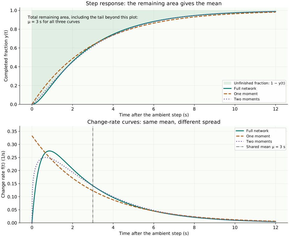
| Model | μ | Variance (s²) | t₁₀ | t₉₀ | Rise time | Rise error |
|---|---|---|---|---|---|---|
| Full two-node response | 3 | 7 | 0.582845 | 6.441122 | 5.858277 | Reference |
| One moment | 3 | 9 | 0.316082 | 6.907755 | 6.591674 | +12.52% |
| Two moments | 3 | 7 | 0.476037 | 6.492216 | 6.016180 | +2.70% |
The extra moment helps for this example, while both fitted rise times remain too long. The exact 50% crossing is 2.224919 s, so the exact mean μ = 3 s is visibly not t₅₀. The explorer reproduces the full response and independently checks it by RK4 time marching.
The two modal time constants are τslow = (3+√5)/2 s and τfast = (3−√5)/2 s. Inverting the two-node transfer function gives:
Set this expression equal to 0.1 and 0.9 and solve numerically. The resulting crossings are shown above. The two modes have different amplitudes; replacing the entire expression with a single unit-amplitude exponential loses that information.
Continue with the general matrix derivation, the 10-node Elmore examples, or the interactive rise-time comparisons.
References: Gupta et al., RC-tree delay and first moments; SciPy gamma distribution and inverse CDF. The two-node calculations and teaching diagrams here are independently derived. See additional resources and Google searches.
02 / COMPARE TWO & TEN NODES
Keep the two-node example above. For a fair comparison of total network properties, give both ladders Rtotal = 2 K/W and Ctotal = 2 J/K, with a +1 K left-boundary step and an insulated right end. Each two-node link and capacity is 1 in SI units; each ten-node link and capacity is 0.2. Equal totals do not imply identical transients: the resistance and storage are distributed differently. These ideal ladders are not, by themselves, a mesh-convergence proof for a particular physical slab.
Mean times at nodes 1–10: [0.40, 0.76, 1.08, 1.36, 1.60, 1.80, 1.96, 2.08, 2.16, 2.20] s.
The endpoint first moment has the compact form μN = Rtotal Ctotal(N+1)/(2N). With the same RC = 4 s, it is 3 s for two nodes and 2.2 s for ten. The corresponding full rise times are 5.858277 s and 3.983057 s. A single time constant RC = 4 s cannot describe both distributed responses.
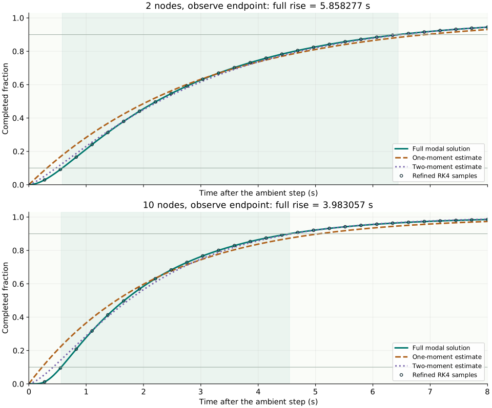
For an interior output, replace the endpoint weight i with min(i,j): wⱼ/xⱼ = 0.04 Σᵢ min(i,j)μᵢ. Downstream capacities still influence upstream nodes through the shared resistances. Apply the same sequence μ → m₂ → σ² → a, θ → crossings:
One-moment rise: 0.878890 s
Two-moment rise: 1.185301 s
Full modal rise: 1.150034 s
One-moment rise: 2.373003 s
Two-moment rise: 2.925186 s
Full modal rise: 2.993823 s
One-moment rise: 3.515559 s
Two-moment rise: 3.710772 s
Full modal rise: 3.680368 s
One-moment rise: 4.833894 s
Two-moment rise: 4.170719 s
Full modal rise: 3.983057 s
Positive errors mean a rise estimate is too long; negative errors mean it is too short. The reference for these percentages is RK4 with the finer time step, not another moment fit.
| Network / observation | μ (s) | One moment (s) | Error | Two moments (s) | Error | Refined RK4 rise (s) |
|---|---|---|---|---|---|---|
| 2 nodes · node 1 | 2.000000 | 4.394449 | -13.32% | 4.995190 | -1.48% | 5.069981 |
| 2 nodes · node 2 | 3.000000 | 6.591674 | +12.52% | 6.016180 | +2.70% | 5.858278 |
| 10 nodes · node 1 | 0.400000 | 0.878890 | -23.58% | 1.185301 | +3.07% | 1.150034 |
| 10 nodes · node 3 | 1.080000 | 2.373003 | -20.74% | 2.925186 | -2.29% | 2.993823 |
| 10 nodes · node 5 | 1.600000 | 3.515559 | -4.48% | 3.710772 | +0.83% | 3.680368 |
| 10 nodes · node 10 | 2.200000 | 4.833894 | +21.36% | 4.170719 | +4.71% | 3.983057 |
Classical fourth-order Runge–Kutta integrates C dT/dt = b−KT directly from zero change. Each threshold is linearly interpolated between its bracketing time steps. The second run halves Δt. The table shows nine decimal places to reveal small numerical differences; these digits do not represent experimentally validated precision.
| Network / observation | Fine t₁₀ (s) | Fine t₉₀ (s) | Modal rise (s) | RK4 rise, Δt (s) | RK4 rise, Δt/2 (s) | Fine − modal (s) | Δt / Δt/2 (s) |
|---|---|---|---|---|---|---|---|
| 2 nodes · node 1 | 0.111321465 | 5.181302713 | 5.069981268 | 5.069979756 | 5.069981248 | -2.022e-08 | 0.002618034 / 0.001309017 |
| 2 nodes · node 2 | 0.582844599 | 6.441122152 | 5.858277400 | 5.858278032 | 5.858277553 | +1.530e-07 | 0.002618034 / 0.001309017 |
| 10 nodes · node 1 | 0.004453605 | 1.154487341 | 1.150034141 | 1.150015465 | 1.150033737 | -4.045e-07 | 0.001790643 / 0.0008953214 |
| 10 nodes · node 3 | 0.063349663 | 3.057172555 | 2.993822887 | 2.993822803 | 2.993822892 | +5.360e-09 | 0.001790643 / 0.0008953214 |
| 10 nodes · node 5 | 0.181822036 | 3.862190206 | 3.680368143 | 3.680368031 | 3.680368169 | +2.630e-08 | 0.001790643 / 0.0008953214 |
| 10 nodes · node 10 | 0.564248217 | 4.547305039 | 3.983056762 | 3.983057104 | 3.983056822 | +5.977e-08 | 0.001790643 / 0.0008953214 |
All six refined RK4 rise times differ from the modal results by less than 0.000001 s. An independent Python calculation using SciPy’s adaptive DOP853 integrator also agrees. Download the comparison data and independent verification script (NumPy and SciPy).
03 / VARY MASSES, LINKS & BOUNDARIES
Use the same ten-node ladder in all five experiments. All nodes start at 25°C. Each capacity represents stored heat, not a mass in kilograms. The right end is either insulated or connected through Rright = 0.25 K/W to a reservoir held at Tfix = 25°C. Node 5 is the chosen middle heat-input node; an even ten-node chain has two central nodes.
R₁ connects Tamb to node 1; Rᵢ for i ≥ 2 connects nodes i−1 and i. The left-to-node-10 resistance totals 2 K/W and total capacity is 2 J/K. With the extra right reservoir, boundary-to-boundary resistance is 2.25 K/W. The larger capacity at node 5 and larger link resistance into node 6 make the storage and transport distribution visibly nonuniform.
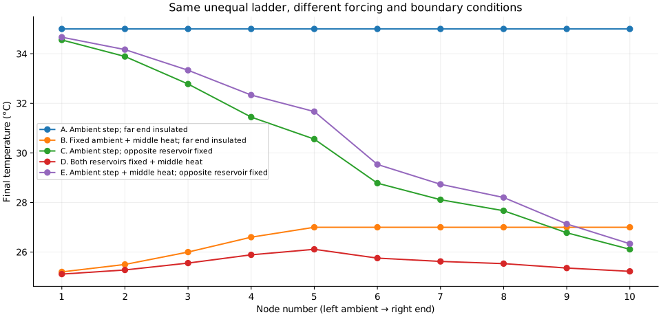
Let Sᵢ be the accumulated resistance from the left reservoir to node i, and Z = K⁻¹. With no right sink, Zⱼᵢ = min(Sⱼ,Sᵢ). With the fixed right reservoir, Zⱼᵢ = min(Sⱼ,Sᵢ) − SⱼSᵢ/(2.25 K/W). For a left-boundary temperature step ΔTamb and a heat step Q at node 5, the forcing has b₁ = ΔTamb/R₁ and an additional b₅ = Q. Add these powers before solving the network.
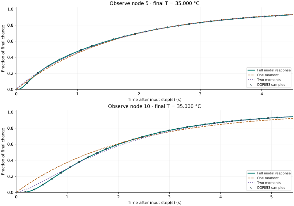
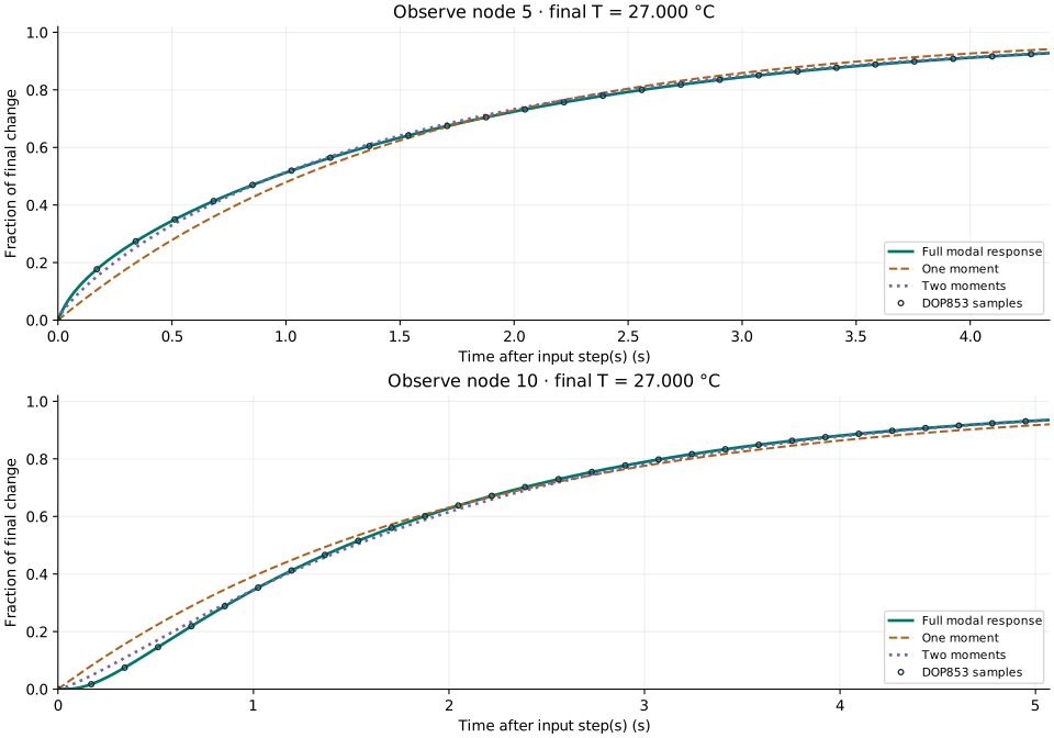
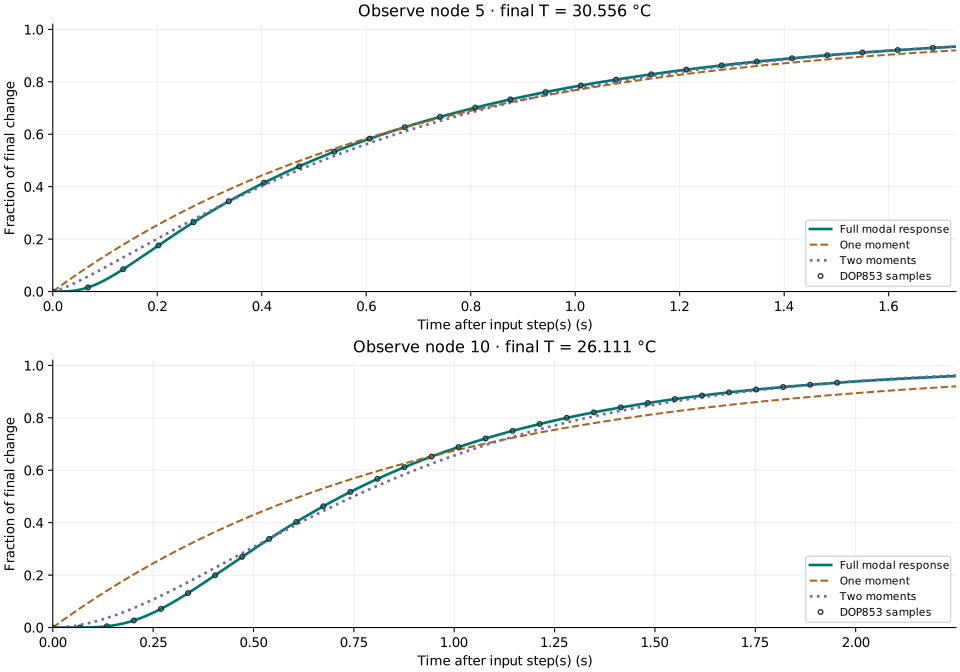
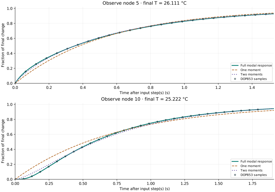
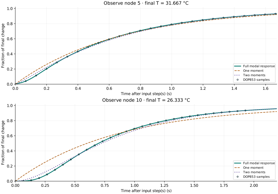
The xᵢ/xⱼ weights are essential when heating occurs internally or the other boundary stays fixed. The response curves show the full modal solution with independent DOP853 samples; tables compare it with RK4 at two step sizes and the two moment estimates.
Tamb steps from 25°C to 35°C; Q = 0; the far end is insulated. Every node eventually reaches 35°C, so all xᵢ = 10 K and the weights xᵢ/xⱼ are one. The shared-path Elmore sum applies directly.
At node 5: μ = 1.668000 s; w₅/x₅ = 2.880830 s²; σ² = 2.979436 s²; gamma shape a = 0.933809, scale θ = 1.786233 s. These are obtained from the same three solves above, with this case’s K and b.
| Node | Final T (°C) | μ | One moment / error | Two moments / error | Full modal rise | Refined RK4 rise |
|---|---|---|---|---|---|---|
| 1 | 35.0000 | 0.200000 | 0.439445+63.95% | 0.422662+57.69% | 0.268035 | 0.268034 |
| 3 | 35.0000 | 0.938000 | 2.060997-26.02% | 2.646371-5.01% | 2.786032 | 2.786032 |
| 5 | 35.0000 | 1.668000 | 3.664971-1.32% | 3.751806+1.02% | 3.714008 | 3.714008 |
| 10 | 35.0000 | 2.143000 | 4.708652+20.30% | 4.089397+4.48% | 3.914121 | 3.914121 |
Tamb is held at 25°C; Q steps from 0 to 2 W at node 5; the far end is insulated. All generated heat eventually leaves through the left boundary. The final change is xⱼ = Q min(Sⱼ,S₅); nodes 5–10 share the same final temperature but have different transients.
At node 5: μ = 1.532300 s; w₅/x₅ = 2.659307 s²; σ² = 2.970672 s²; gamma shape a = 0.790375, scale θ = 1.938701 s. These are obtained from the same three solves above, with this case’s K and b.
| Node | Final T (°C) | μ | One moment / error | Two moments / error | Full modal rise | Refined RK4 rise |
|---|---|---|---|---|---|---|
| 1 | 25.2000 | 1.668000 | 3.664971-1.32% | 3.751806+1.02% | 3.714008 | 3.714008 |
| 3 | 26.0000 | 1.646600 | 3.617950-2.59% | 3.735729+0.59% | 3.713974 | 3.713974 |
| 5 | 27.0000 | 1.532300 | 3.366807-9.17% | 3.638148-1.85% | 3.706906 | 3.706906 |
| 10 | 27.0000 | 2.007300 | 4.410489+12.89% | 4.024772+3.02% | 3.906752 | 3.906752 |
Tamb steps from 25°C to 35°C while Tfix stays at 25°C; Q = 0. The final profile is xⱼ = 10[1−Sⱼ/(2.25 K/W)] K. The right boundary removes heat and changes both the matrix K and the final-output normalization.
At node 5: μ = 0.684222 s; w₅/x₅ = 0.417617 s²; σ² = 0.367074 s²; gamma shape a = 1.275383, scale θ = 0.536484 s. These are obtained from the same three solves above, with this case’s K and b.
| Node | Final T (°C) | μ | One moment / error | Two moments / error | Full modal rise | Refined RK4 rise |
|---|---|---|---|---|---|---|
| 1 | 34.5556 | 0.068213 | 0.149879+37.77% | 0.160834+47.84% | 0.108787 | 0.108787 |
| 3 | 32.7778 | 0.345422 | 0.758970-19.50% | 0.941183-0.17% | 0.942782 | 0.942782 |
| 5 | 30.5556 | 0.684222 | 1.503390+13.34% | 1.376334+3.76% | 1.326411 | 1.326411 |
| 10 | 26.1111 | 0.890422 | 1.956458+39.94% | 1.485290+6.24% | 1.398048 | 1.398048 |
Tamb and Tfix both stay at 25°C; Q steps from 0 to 2 W at node 5. Heat can leave through both boundaries. The final change is xⱼ = Q Zⱼ₅. This isolates the effect of adding middle-node heating while holding both reservoir temperatures fixed.
At node 5: μ = 0.548522 s; w₅/x₅ = 0.329593 s²; σ² = 0.358310 s²; gamma shape a = 0.839711, scale θ = 0.653227 s. These are obtained from the same three solves above, with this case’s K and b.
| Node | Final T (°C) | μ | One moment / error | Two moments / error | Full modal rise | Refined RK4 rise |
|---|---|---|---|---|---|---|
| 1 | 25.1111 | 0.684222 | 1.503390+13.34% | 1.376334+3.76% | 1.326411 | 1.326411 |
| 3 | 25.5556 | 0.662822 | 1.456369+9.86% | 1.364963+2.96% | 1.325673 | 1.325673 |
| 5 | 26.1111 | 0.548522 | 1.205227-6.90% | 1.277663-1.31% | 1.294565 | 1.294565 |
| 10 | 25.2222 | 0.754722 | 1.658294+20.81% | 1.428457+4.07% | 1.372635 | 1.372635 |
Tamb steps from 25°C to 35°C and Q simultaneously steps from 0 to 2 W at node 5; Tfix stays at 25°C. Unnormalized temperature changes from cases C and D add by linear superposition. Their normalized rise times do not add: normalize the summed response and then find its crossings.
At node 5: μ = 0.661606 s; w₅/x₅ = 0.402946 s²; σ² = 0.368171 s²; gamma shape a = 1.188909, scale θ = 0.556481 s. These are obtained from the same three solves above, with this case’s K and b.
| Node | Final T (°C) | μ | One moment / error | Two moments / error | Full modal rise | Refined RK4 rise |
|---|---|---|---|---|---|---|
| 1 | 34.6667 | 0.075293 | 0.165437+29.01% | 0.185363+44.55% | 0.128237 | 0.128237 |
| 3 | 33.3333 | 0.366582 | 0.805463-18.53% | 0.984119-0.46% | 0.988664 | 0.988664 |
| 5 | 31.6667 | 0.661606 | 1.453696+9.38% | 1.366253+2.80% | 1.328989 | 1.328989 |
| 10 | 26.3333 | 0.867806 | 1.906764+36.12% | 1.481034+5.73% | 1.400747 | 1.400747 |
Fine Δt is half the coarse step. Threshold crossings are interpolated between time levels. The final column comes from a separate adaptive SciPy integrator. Numerical agreement validates these linear model calculations, not a real material or device.
| Case / output | Modal rise | Coarse RK4 | Fine RK4 | Fine − modal (s) | Fine Δt (s) | DOP853 rise |
|---|---|---|---|---|---|---|
| ambient-free · node 1 | 0.268034533 | 0.268032984 | 0.268034183 | -3.499e-07 | 0.0001303629 | 0.268034533 |
| ambient-free · node 3 | 2.786032052 | 2.786032044 | 2.786032050 | -2.274e-09 | 0.0001303629 | 2.786032052 |
| ambient-free · node 5 | 3.714008427 | 3.714008427 | 3.714008428 | +6.502e-10 | 0.0001303629 | 3.714008427 |
| ambient-free · node 10 | 3.914120889 | 3.914120898 | 3.914120890 | +1.297e-09 | 0.0001303629 | 3.914120889 |
| heat-free · node 1 | 3.714008427 | 3.714008427 | 3.714008428 | +6.502e-10 | 0.0001303629 | 3.714008427 |
| heat-free · node 3 | 3.713974490 | 3.713974489 | 3.713974489 | -8.043e-10 | 0.0001303629 | 3.713974490 |
| heat-free · node 5 | 3.706905753 | 3.706905735 | 3.706905743 | -9.292e-09 | 0.0001303629 | 3.706905753 |
| heat-free · node 10 | 3.906752235 | 3.906752242 | 3.906752237 | +1.538e-09 | 0.0001303629 | 3.906752235 |
| ambient-fixed · node 1 | 0.108786561 | 0.108786014 | 0.108786544 | -1.634e-08 | 7.595312e-05 | 0.108786561 |
| ambient-fixed · node 3 | 0.942781950 | 0.942781960 | 0.942781954 | +3.975e-09 | 7.595312e-05 | 0.942781950 |
| ambient-fixed · node 5 | 1.326410665 | 1.326410670 | 1.326410667 | +1.538e-09 | 7.595312e-05 | 1.326410665 |
| ambient-fixed · node 10 | 1.398047678 | 1.398047685 | 1.398047681 | +2.554e-09 | 7.595312e-05 | 1.398047678 |
| heat-fixed · node 1 | 1.326410665 | 1.326410670 | 1.326410667 | +1.538e-09 | 7.595312e-05 | 1.326410665 |
| heat-fixed · node 3 | 1.325672865 | 1.325672871 | 1.325672867 | +2.252e-09 | 7.595312e-05 | 1.325672865 |
| heat-fixed · node 5 | 1.294564983 | 1.294564971 | 1.294564978 | -5.136e-09 | 7.595312e-05 | 1.294564983 |
| heat-fixed · node 10 | 1.372635134 | 1.372635141 | 1.372635137 | +2.447e-09 | 7.595312e-05 | 1.372635134 |
| combined-fixed · node 1 | 0.128237172 | 0.128236617 | 0.128237130 | -4.207e-08 | 7.595312e-05 | 0.128237172 |
| combined-fixed · node 3 | 0.988664319 | 0.988664331 | 0.988664323 | +3.532e-09 | 7.595312e-05 | 0.988664319 |
| combined-fixed · node 5 | 1.328988900 | 1.328988906 | 1.328988903 | +2.702e-09 | 7.595312e-05 | 1.328988900 |
| combined-fixed · node 10 | 1.400746533 | 1.400746544 | 1.400746536 | +2.932e-09 | 7.595312e-05 | 1.400746533 |
Download the complete case data · Download independent verification (NumPy + SciPy)
04 / EXPLORE YOUR OWN NETWORK
All nodes start at zero temperature change. Apply a boundary temperature step or a constant heat-input step. Temperatures are changes from the initial equilibrium; material properties stay constant.
The two exponential curves are comparison approximations with unit amplitude. The actual response includes all mode amplitudes.
| Output | ln(9)μ estimate (s) | Two-moment estimate (s) | Modal rise (s) | RK4 rise (s) | RK4 Δt (s) |
|---|
| Node | ΔT steady (K) | μ (s) | t₁₀ (s) | t₅₀ (s) | t₆₃.₂ (s) | t₉₀ (s) | 10–90% (s) |
|---|
First solve Kx = b for the steady temperature change x. Then solve Kv = Cx. At output j, μⱼ = vⱼ/xⱼ = Σᵢ (K⁻¹)ⱼᵢ Cᵢ xᵢ/xⱼ. This handles both reservoirs and internal heat input without misusing a single-sink path rule.
| i | (K⁻¹)ⱼᵢ (K/W) | Cᵢ (J/K) | xᵢ/xⱼ | Contribution (s) |
|---|
K has negative link conductances off the diagonal. Its diagonal includes every connected link, including reservoir links. C is diagonal. Rates are eigenvalues of C⁻½KC⁻½, which is symmetric and similar to C⁻¹K.
05 / GO DEEPER
Open a topic when you need another derivation, a practical estimate, or a different network.
02 / THE PHYSICS
For a uniform-temperature body with constant conductance to a reservoir:
With constant Q, Tsteady = T∞ + Q/G. At τ, 63.212% of the change is complete. At 3τ, 95.02%; at 5τ, 99.33%. The 10–90% rise time is ln(9)τ ≈ 2.197τ.
For external convection, G = hA and C = ρVcp. A common lumped-body criterion is Bi = h(V/A)/k < 0.1; check internal gradients and actual geometry. BYU heat-transfer notes ↗
α has units m²/s. For a slab of area A and thickness L, R = L/(kA) and C = ρcpAL, so RC = L²/α. This is a scale, not a universal threshold time.
A homogeneous slab held at one face and insulated at the other has dominant τ = 4L²/(π²α). If both faces are held fixed and L is the full thickness, τ = L²/(π²α). Boundary conditions and the observation point matter.
Adding “diffusion time” to “bulk rise time” is not a general model: both may account for the same distributed storage. Derive the combined network instead. A separate physical boundary resistance can legitimately add a term to the first moment.
Positive capacities and reciprocal passive conductances produce real, nonnegative decay rates. With each connected component linked to a fixed-temperature reservoir, all rates are positive. An isolated network has a zero mode: its mean temperature does not relax to a prescribed ambient.
There can be repeated rates. A slow mode may be weak or invisible for a particular forcing and sensor. The slowest network mode alone does not give every node’s rise time. Passive networks can contain geometric loops; reciprocal conduction does not prohibit loops.
The moment is exact for the stated model; using it as a threshold time is an approximation. Neither t₅₀ = μ − 0.35σ nor t₁₀–₉₀ = 2.2σ is a universal identity. Compute the full response when thresholds matter. Gupta et al., Elmore delay bounds ↗
Here, threshold delay t₅₀ measures time from the applied step to 50% of the final temperature change. Elmore / first-moment delay μ is the area above the normalized step response. Rise time tᵣ = t₉₀ − t₁₀ measures the transition between 10% and 90%. A pure transport delay shifts both crossing times equally and leaves this rise time unchanged.
Fractions are relative to the initial-to-final temperature change. These formulas also describe cooling when the response is normalized this way. A constant heat input changes the final temperature but not τ in this linear model.
This fits one exponential using the first moment. It is exact for a single RC model and an estimate for a multi-node network. It can overpredict rise time because part of μ represents a delayed onset. For internal heat input or multiple sinks, use the normalized matrix expression above for μ.
A practical refinement fits a gamma-shaped impulse response using the exact mean μ and variance σ². Define shape a = μ²/σ² and scale θ = σ²/μ. If P(a,z) is the regularized lower incomplete gamma function, the estimated normalized step is y(t) ≈ P(a,t/θ).
The browser evaluates the inverse numerically. With one lumped capacitance, a = 1 and θ = τ, recovering ln(9)τ exactly. For a narrow, nearly Gaussian impulse shape, a rough width estimate is 2.563σ; for a single exponential it is 2.197σ. Neither coefficient is universal. The gamma fit is a moment-matching approximation, not a guaranteed bound or an exact multi-node solution; inspect its error against time marching below.
FOUNDATIONS / HEAT BALANCE → TEMPERATURE RESPONSE → TIMING
A thermal response has no single universal “response time.” We first derive the temperature history, then define the timing quantity we want to extract. In this section time is measured from an ideal input step at t = 0. Temperatures refer to a stationary solid, with no bulk fluid advection or phase change.
A. Heat equation · B. Lumped model · C. Delay versus rise time · D. A true delay · E. Distributed networks
1. Balance a small fixed control volume. Let q be the conductive heat-flux vector (W/m²), q̇ᵥ the volumetric heat generation (W/m³), ρ the density (kg/m³), and cₚ the specific heat capacity (J/(kg·K)). Stored thermal energy increases through heat generation and net inward conduction:
For constant isotropic conductivity k and constant ρcₚ, this becomes ∂T/∂t = α∇²T + q̇ᵥ/(ρcₚ), where α = k/(ρcₚ). All terms in the energy equation have units W/m³. If k varies spatially, retain ∇·(k∇T); do not replace it by k∇²T without justification.
2. Specify initial and boundary conditions. The differential equation alone cannot determine a time response. Typical choices, with outward surface normal n, are:
A prescribed-temperature boundary and convection through a finite h are different models. For a slab with coordinate ξ = x/L and dimensionless time Fo = αt/L², the source-free equation becomes ∂T/∂Fo = ∂²T/∂ξ². This identifies L²/α as the diffusion time scale. A threshold time also depends on the dimensionless solution, boundary conditions, and sensor location.
1. Integrate over the body. Applying the divergence theorem gives an exact global balance for constant properties:
Here Q(t) = ∫ᵥq̇ᵥdV is total internal heating in watts; insulated surfaces contribute zero outward heat flow. The surface integral is over the heat-exchanging surface. A volume-averaged temperature alone does not close this exact equation because the surface temperature can differ from the average.
2. Make the lumped approximation. When internal gradients are small, approximate T(r,t) ≈ T(t), including at the surface. Define Cth = ∫ᵥρcₚdV = ρcₚV for a homogeneous body. For a common ambient temperature and constant h, G = hAₛ. More generally G = ∫ₛh dA if the same ambient acts over the surface:
Every term now has units W. The capacity Cth is in J/K, not kilograms: mass m must be multiplied by cₚ. Several independent conductances to fixed reservoirs contribute Gtotal = ΣGₗ and forcing ΣGₗTₗ + Q, giving τ = Cth/Gtotal. Resistances in a series path combine before taking its reciprocal.
3. Check when the approximation is sensible. For convection, choose Lc = V/Aₛ and define Bi = hLc/k. Comparing scales based on that same Lc:
Small Bi means internal equilibration is fast compared with exchange with the surroundings. Bi < 0.1 is a common engineering screening criterion, not an error guarantee for every geometry, local heat source, or material arrangement. The approximation is obtained from the integrated energy balance; setting ∇²T = 0 in the local equation and then discarding the boundary flux would incorrectly eliminate the mechanism that heats or cools the body. MIT: transient heat transfer and the lumped approximation ↗
4. Solve the post-step ordinary differential equation. For constant T∞, Q, and G > 0 after t = 0, set dT/dt = 0 to find Tss = T∞ + Q/G. Let z(t) = T(t)−Tss. Substitution removes the constant forcing:
For z(0) = 0, the solution is already at equilibrium and there is no transition. With a nonzero final change, normalize progress as y(t) = [T(t)−T₀]/[Tss−T₀]. This definition gives y(0) = 0 and y(∞) = 1 for both heating and cooling:
For a body with no heat-loss path (G = 0), constant nonzero Q instead gives T(t) = T₀ + Qt/Cth. There is no finite steady temperature, so the steady-state percentage rise-time formulas do not apply.
Threshold delay tₚ is the elapsed time from the input step to the first crossing y = p. In a monotone response the crossing is unique. A common convention is tdelay = t₅₀, but every report should name its threshold. Solving the lumped response gives:
Rise time is the duration between two selected crossings, not the elapsed time from the input step. For fractions p₁ < p₂:
Elmore / mean delay μ uses the complete response instead of one crossing. For the normalized lumped model, the impulse response is f(t) = dy/dt = e−t/τ/τ. Its first moment, using integration by parts, is:
Equivalently μ = ∫₀∞[1−y(t)]dt. Thus μ equals τ for this one-pole response, while t₅₀ and t₁₀–₉₀ do not. The standard deviation of this impulse response is also τ, since ∫t²f(t)dt = 2τ² and σ² = 2τ²−τ².
| Quantity | Definition | Single lumped RC |
|---|---|---|
| Threshold delay | Time from input step to 50% | t₅₀ = 0.693147τ |
| Elmore delay | Mean impulse time / remaining area | μ = τ |
| Time constant | Exponential decay scale | t₆₃.₂₁₂… = τ |
| 10–90% rise time | Duration from 10% to 90% | tr = 2.197225τ |
| 2% settling time | Remaining error ≤ 2%, thereafter | ts = −τ ln(0.02) ≈ 3.912023τ |
The phrase “rise time to 63.2%” sometimes means an elapsed response time, but it is not the 10–90% rise time used here. A pure exponential never reaches exactly 100% at a finite time; always specify a settling tolerance. For nonmonotone systems, first-crossing times and settling time need additional care because a response can cross a threshold more than once.
Suppose the applied input is postponed by a known time d before reaching the same lumped body. This is an imposed transport or actuation delay, not an automatic property of Fourier conduction. Solving the ODE before and after the delayed step gives:
The extra d appears in both thresholds and cancels in their difference. In contrast, the mean delay includes the rectangle of height one and width d before the response starts:
The variance stays the same because shifting a distribution changes its mean but not its width. If the response is known to be a delayed single exponential, its moments imply τ = σ, d = μ−σ (requiring μ ≥ σ), and tr = ln(9)σ. This is a different shape assumption from the gamma fit; it is not a general network identity, and μ−σ must not be interpreted automatically as physical transport delay.
Take Cth = 100 J/K and G = 5 W/K, so τ = 20 s. The boundary steps from 20°C to 80°C, with Q = 0. The 10%, 50%, and 90% temperatures are 26°C, 50°C, and 74°C. For cooling from 80°C to 20°C, they would be 74°C, 50°C, and 26°C, with identical normalized timing.
| Metric | Immediate input | Input delayed by 10 s |
|---|---|---|
| t₁₀ | 2.10721 s | 12.10721 s |
| t₅₀ threshold delay | 13.86294 s | 23.86294 s |
| t₉₀ | 46.05170 s | 56.05170 s |
| Elmore delay μ | 20 s | 30 s |
| 10–90% rise time | 43.94449 s | 43.94449 s |
Divide the body into control volumes. Integrate the energy equation over each volume, approximate its temperature by Tᵢ, and replace each conductive face flux by a conductance times the adjacent temperature difference. For a uniform connecting segment, Gᵢⱼ = kA/ℓ; for unequal cell-center layers, add the two half-layer resistances and any contact resistance before inverting.
Internal fluxes cancel when all node balances are added, which preserves total energy. Kᵢᵢ is the sum of all conductances out of node i, including boundary links, and Kᵢⱼ = −Gᵢⱼ. With constant post-step forcing, solve KTss = b. The error z = T−Tss then satisfies C dz/dt = −Kz.
For a nonzero transition at node j, Aⱼₖ = −aₖφⱼₖ/(Tss,ⱼ−T₀,ⱼ), and ΣₖAⱼₖ = 1. These coefficients depend on the initial state, forcing, and observation point; individual coefficients need not all be positive even for a monotone response. Thresholds must solve ΣₖAⱼₖe−tₚ/τₖ = 1−p, generally numerically. But the remaining-area definition integrates term by term:
This explains why neither the slowest τₖ nor the exact μⱼ automatically equals a threshold delay or rise time. The derivations below obtain these same moments by linear solves, then explicitly choose a one-pole or gamma approximation to estimate rise time.
Diffusion is not a literal waiting period. The classical Fourier heat equation is parabolic. Its ideal mathematical solution generally has an arbitrarily small response at a remote point for any t > 0; it does not create a sharp finite arrival time. A practical “diffusion delay” therefore needs a specified threshold or measurement resolution. Treating L²/α as an exact dead time and then adding a bulk RC rise time can count the same storage twice. Finite-speed or non-Fourier models are outside this page’s scope.
DERIVATION / FROM THE NETWORK TO RISE TIME
For a gentler introduction with every step worked out, start with Why the estimates work and its two- and ten-node examples.
Both estimates begin with exact moments of the selected input-to-temperature response. The approximation enters only when we choose a response shape from those moments. Below, C is the diagonal matrix of node heat capacities, K is the grounded conductance matrix, b is the forcing vector for a unit input, and eⱼ selects observation node j.
Start with the heat equation and timing definitions ↑
1. Exact network moments · 2. Elmore-based rise time · 3. Two-moment rise time · 4. Worked 10-node example
Step 1 — Transform the heat balance. With input u(t), the thermal network obeys C dT/dt + KT = bu(t). Taking a Laplace transform at zero initial conditions gives:
For a unit step, let x = K⁻¹b be the steady temperature-change vector. Thus Hⱼ(0) = xⱼ. Normalize the transfer function as Fⱼ(s) = Hⱼ(s)/xⱼ, and the unit-step response as yⱼ(t) = Tⱼ(t)/xⱼ. Then Fⱼ(0) = 1 and yⱼ(∞) = 1.
Step 2 — Expand the inverse without changing matrix order. Factor K + sC = K(I + sK⁻¹C), and use the geometric series near s = 0:
Define three successive linear solves. They use the same K, so a matrix factorization can be reused:
Step 3 — Identify the moments. Let fⱼ(t) = dyⱼ/dt be the normalized impulse response. It integrates to one. Expand its Laplace integral directly:
The factor of two is essential: the coefficient of s² is half the second raw moment, not the moment itself. μ has units seconds, m₂ and σ² have units seconds squared. The coefficient wⱼ/xⱼ belongs to the normalized transfer-function expansion; it is not generally a denominator coefficient.
Step 4 — Connect the first moment to step-response delay. Since f = y′ = −(1−y)′, integration by parts gives μ = [−t(1−y)]₀∞ + ∫₀∞(1−y)dt. The boundary term vanishes for a stable finite RC network. Similarly, m₂ = 2∫₀∞t(1−y)dt.
Thus μ measures the total area remaining above the normalized response. It is not defined as a particular crossing time. These integrals also provide a way to estimate moments from a sufficiently long measured or time-marched response, with care for the unobserved tail.
Step 1 — Reduce the matrix expression to shared paths. Write Z = K⁻¹. Then:
For a tree with one stepped reservoir and no other sink, the final temperature change is identical at every node, so xᵢ/xⱼ = 1. To interpret Zⱼᵢ, inject one watt at node i while the root reservoir is held at zero temperature change. That watt flows along the unique path from i to the root. The temperature at node j equals the sum of resistances on the part shared by the root-to-i and root-to-j paths. Therefore Zⱼᵢ = Rshared(i,j):
The second form follows by exchanging the sums: each edge carries the contribution of all capacities downstream of it, including branches. With several sinks or local heat input, retain Zⱼᵢ and the steady-state weights xᵢ/xⱼ; an unweighted shared-path sum is not generally valid.
Step 2 — Fit a single pole to the first moment. Choose F₁(s) = 1/(1+sτfit). Its expansion is 1−sτfit+s²τfit²−… . Matching the exact constant and first-order terms forces τfit = μ:
Step 3 — Solve for the thresholds. Set y₁(tₚ) = p, so e−tₚ/μ = 1−p. Subtract the two threshold times:
This also predicts t₅₀,1 = μ ln(2). Calling μ itself a “delay estimate” does not make μ the exact t₅₀. The rise-time formula is exact for a single lumped RC; for a network it is the consequence of an explicitly chosen one-pole fit.
Why one moment is insufficient. A pure delay d followed by a single RC has F(s) = e−sd/(1+sτ), μ = d+τ, and σ² = τ². Its actual 10–90% rise time is ln(9)τ because the delay cancels in the difference. The one-moment estimate ln(9)(d+τ) counts that delay as extra rise duration. This example explains the limitation; a diffusion network need not have a literal dead-time segment.
Step 1 — Choose a positive two-parameter shape. Mean and variance do not uniquely determine a waveform, so a shape assumption is still needed. This page chooses the gamma impulse-response family:
Here a is dimensionless and θ is a time scale. Substituting z = t/θ verifies ∫f₂dt = 1. Applying the same substitution to ∫tᵏf₂dt gives θᵏΓ(a+k)/Γ(a). Using Γ(a+1) = aΓ(a):
Step 2 — Match the exact network moments. Equating aθ = μ and aθ² = σ², first divide the second equation by the first, then solve for a:
Equivalently, the gamma transfer function is F₂(s) = (1+sθ)−a. Its expansion is 1−aθs+[a(a+1)θ²/2]s²−… . Substitution yields 1−μs+[(μ²+σ²)/2]s²−… , matching the exact network through s². This is a two-moment fit; it is not necessarily a two-pole model. A noninteger a generally does not correspond to a finite rational RC transfer function.
Step 3 — Integrate to obtain the step response. Define the regularized lower incomplete gamma function P(a,z). Then:
Step 4 — Invert the thresholds. P⁻¹(a,p) denotes the nonnegative z satisfying P(a,z) = p; it is an inverse in the second argument, not 1/P. Consequently:
The inverse is evaluated numerically. For an independent calculation, use gamma.ppf(p, a, scale=theta) in SciPy, with zero location. The SciPy gamma reference defines the distribution and its inverse CDF. Choosing this family is an approximation made here, not a universal Elmore rise-time theorem.
Step 5 — Check the single-node limit. A single RC gives F(s) = 1/(1+sτ), μ = τ, m₂ = 2τ², and σ² = τ². Therefore a = 1 and θ = τ. Since Γ(1) = 1 and P(1,z) = 1−e−z, the two-moment formula reduces exactly to τ ln(9).
Step 6 — Understand the limits. If a is large, the gamma shape approaches a normal shape with mean μ and standard deviation σ, giving tᵣ ≈ [Φ⁻¹(0.9)−Φ⁻¹(0.1)]σ ≈ 2.563103σ. For a = 1, the factor is ln(9) ≈ 2.197225. For other shapes neither constant is exact. If a < 1, the fitted impulse response is singular at t = 0 even though a finite RC network has a finite initial derivative; this can limit early-time accuracy. Matching two moments does not fix skewness, a separate transport delay, or the long-time decay rate. The estimate can be high or low and has no general error bound.
Use the default left-step / insulated-end ladder: N = 10, each r = 0.1 K/W, each c = 0.1 J/K, and observe node 10. A unit boundary step gives xᵢ = 1 K. Here Zⱼᵢ = r min(i,j), so the complete first-moment vector is:
At the last node, the first solve gives μ₁₀ = 0.01(1+2+…+10) = 0.55 s. For the second solve, use vᵢ = xᵢμᵢ and sum the same inverse-matrix row again:
One moment gives tᵣ,1 = ln(9)(0.55) = 1.208474 s. Two moments give a = 0.55²/0.2035 = 1.486486 and θ = 0.2035/0.55 = 0.370000 s. The gamma quantiles are:
The full modal solution gives t₁₀ = 0.141062 s and t₉₀ = 1.136826 s, hence tᵣ = 0.995764 s. Refined RK4 time marching agrees to the displayed six decimals. The one-moment estimate is about 21.36% high; the two-moment estimate is about 4.71% high. Notice that a reasonably close rise-time difference does not imply that both individual threshold times are equally accurate.
Compare the other examples and time-step refinement below ↓ · Inspect the selected node’s individual moment contributions ↑
PHYSICAL LAYERS → THERMAL CIRCUIT
Consider air heating a copper plate, followed by an insulating polymer and a sensor. The far face of the sensor is insulated. Each node stores the heat capacity of its entire layer, while its temperature represents the layer center. Assume one-dimensional conduction, common cross-sectional area A, constant properties, and perfect contact between layers.
Rᵢ in K/W; thickness Lᵢ in m; conductivity kᵢ in W/(m·K); area A in m². This is the full-layer resistance.
Cᵢ in J/K; density ρᵢ in kg/m³; volume Vᵢ in m³; specific heat cₚ,ᵢ in J/(kg·K).
Rconv in K/W; heat-transfer coefficient h in W/(m²·K). Here the exposed face has area A; use the actual exposed area if different.
Fourier’s law gives Q̇ = kA(Tleft−Tright)/L, hence R = ΔT/Q̇ = L/(kA). A uniform half-layer has half that resistance. Newton’s convection law gives Q̇ = hA(Tamb−Tsurface), hence Rconv = 1/(hA).
Add an interface contact resistance to its corresponding inter-node link if needed. A right convective boundary would add r₃b = R₃/2 + 1/(hright Aright); it would change the topology and require the general matrix moment formula instead of the single-sink sum below.
Each complete intervening layer contributes its full resistance; the observed layer contributes only the half between its center and the previous interface. These paths describe a lumped approximation to the geometry, not an exact spatial temperature field inside each layer.
Apply a step in Tamb with no internal heat generation and no other sink. At steady state, every node has the same temperature change, so xᵢ/x₃ = 1. The common path from node i and node 3 back to ambient has resistance Sᵢ. The general moment formula therefore reduces to:
This expansion shows how convection loads all capacities, whereas each downstream resistance affects a smaller subset. Equivalently μ₃ = r₀₁(C₁+C₂+C₃) + r₁₂(C₂+C₃) + r₂₃C₃. At an upstream observation node j, the correct shared resistance is Smin(i,j), so μⱼ = Σᵢ Smin(i,j)Cᵢ.
For continuity with the existing unequal-layer preset, use illustrative full-layer resistances R = [0.005, 2.5, 0.1] K/W, capacities C = [3.5, 0.8, 0.2] J/K, and Rconv = 0.5 K/W. These are circuit inputs for an example, not certified copper, polymer, or sensor material data.
| Node | Link into node (K/W) | Accumulated Sᵢ (K/W) | Cᵢ (J/K) | SᵢCᵢ (s) |
|---|---|---|---|---|
| 1 · Copper | 0.5 + 0.005/2 = 0.5025 | 0.5025 | 3.5 | 1.75875 |
| 2 · Polymer | 0.005/2 + 2.5/2 = 1.2525 | 1.755 | 0.8 | 1.404 |
| 3 · Sensor | 2.5/2 + 0.1/2 = 1.3 | 3.055 | 0.2 | 0.611 |
For the same input and sensor, the two-moment estimate is about 6.71640 s; the full modal solution and RK4 time marching give about 6.47804 s. The one-moment estimate is about 28.00% high and the two-moment estimate about 3.68% high. The explorer shows the full transient, all node times, and individual moment contributions.
The last equation has no heat-loss term at the insulated face. These are the equations solved by the explorer after the full-layer resistances have been converted into center-to-center links.
Active controllers require an augmented dynamic model. For a single pole H(s) = K₀/(1+sτ) with proportional negative feedback gain Kc, the closed-loop pole has τ/(1+KcK₀). This shortcut does not apply to an arbitrary multi-node network or a controller with its own dynamics.
WORKED GUIDE / A SHORTCUT YOU CAN CALCULATE BY HAND
For the last node of a 1D chain driven by one ambient-temperature step, with the far end insulated and no other sink, a useful single response metric is:
For a unit ambient step, each node eventually changes by one kelvin. Its capacity contributes to the transient storage, and each upstream resistance restricts heat exchange with that storage. In the first-moment equation Kv = C1, the capacity values act mathematically like steady forcing values. The flow through a given edge is the sum of capacities downstream of that edge. Summing the resulting resistance-times-capacity drops to the endpoint gives:
Here Rₑ denotes an actual circuit link, not a full physical layer. The last line is the accumulated-resistance formula. It results from exchanging the order of summation—not from waiting for one layer to finish warming before the next starts. All nodes evolve simultaneously.
The shared path ends at the nearer of nodes i and k. A downstream capacity still affects an upstream sensor, but only through the common upstream resistances. For a uniform chain of N nodes, with each link r and each capacity c:
Let N = 10, r = 0.1 K/W, and c = 0.1 J/K. The left ambient steps by 1 K; the right end is insulated. Thus Rtotal = 1 K/W and Ctotal = 1 J/K. The following values are first moments; the explorer separately computes threshold and rise times.
All ten capacities share the first resistance.
Node 1 shares one link; node 2 shares two. Nodes 3–10 share three links with the target.
Nodes 1–4 have shorter shared paths. All six nodes 5–10 share five links.
Every node’s full path to ambient is shared with the endpoint.
The endpoint arithmetic progression gives the closed form:
To turn this into a one-pole rise-time estimate, multiply μ by ln(9): the endpoint estimate is 1.20847 s, while its actual 10–90% rise time is 0.995764 s. The agreement of μ with a particular t₆₃.₂ in one example is not a general equality.
Keep N = 10 and r = c = 0.1 in SI units. A second boundary adds an eleventh resistor, so the boundary-to-boundary resistance is now 1.1 K/W. Let Z = K⁻¹. For a single left reservoir Zₖᵢ = r min(i,k); for two fixed reservoirs:
Z is the steady thermal response to a unit heat injection. For two sinks it is not a unique shared-path resistance. The xᵢ/xₖ factors account for nonuniform final temperature changes. These are the missing factors when applying the endpoint shortcut to a local heat source.
Every entry is Z₅ᵢ Cᵢ xᵢ/x₅, in seconds. The two-step boundary case has xᵢ/x₅ = 1. Values are rounded for display; totals use unrounded values.
| i | Left step, right fixed | Both ends stepped | Q at 5, two sinks | Q at 5, one sink |
|---|---|---|---|---|
| 1 | 0.009091 | 0.005455 | 0.001091 | 0.002000 |
| 2 | 0.016364 | 0.010909 | 0.004364 | 0.008000 |
| 3 | 0.021818 | 0.016364 | 0.009818 | 0.018000 |
| 4 | 0.025455 | 0.021818 | 0.017455 | 0.032000 |
| 5 | 0.027273 | 0.027273 | 0.027273 | 0.050000 |
| 6 | 0.018939 | 0.022727 | 0.018939 | 0.050000 |
| 7 | 0.012121 | 0.018182 | 0.012121 | 0.050000 |
| 8 | 0.006818 | 0.013636 | 0.006818 | 0.050000 |
| 9 | 0.003030 | 0.009091 | 0.003030 | 0.050000 |
| 10 | 0.000758 | 0.004545 | 0.000758 | 0.050000 |
| Total μ₅ | 0.141667 | 0.150000 | 0.101667 | 0.360000 |
The explorer presets reproduce these cases and provide the full transient. The comparison tables below distinguish first moment, dominant mode, actual t₆₃.₂, and 10–90% rise time, including independent time marching. Positive passive-network contributions here do not become negative near the far boundary.
WORKED GUIDE / FROM DELAY TO TRANSITION DURATION
This companion to the Elmore delay guide uses the same 10-node chain and observation nodes. A first moment tells us an average response time; rise time measures the width of a specific transition. The two are connected only after choosing a response shape.
Use each output’s own initial and final temperatures. For warming from 20°C to 30°C, the crossings are 21°C and 29°C. For cooling from 30°C to 20°C, they are 29°C and 21°C.
Exact for a single RC. For a network, this is an approximation based on the exact first moment, not an exact threshold formula.
Subtract the gamma fit’s two crossings. The fit matches mean and variance; it does not guarantee the correct waveform or an upper/lower bound.
Take R = 1 K/W and C = 1 J/K. Then τ = RC = μ = 1 s, σ² = 1 s², a = 1, and θ = 1 s. The gamma shape is an exponential, so both estimates give the exact answer:
Use N = 10, link resistance r = 0.1 K/W, and capacity c = 0.1 J/K per node. The left reservoir steps by 1 K and the right end is insulated. From the Elmore guide, all xᵢ = 1 K and:
The final sum runs over all ten nodes. It is the second linear solve, not a sum of node rise times. The coefficient 0.01 has units seconds; multiplying it by μᵢ produces seconds squared. For example, at node 1, w₁/x₁ = 0.01(0.10 + 0.19 + … + 0.55) = 0.038500 s².
Start with the Elmore calculation: μ1 = 0.100 s.
One moment: ln(9) × 0.100 = 0.219722 s.
Two moments: θ[P⁻¹(a,0.9) − P⁻¹(a,0.1)] = 0.296325 s.
Full response: 0.288622 − 0.001113 = 0.287509 s.
Rise-time errors: one moment -23.58%; two moments +3.07%.
The early response is fast but the long tail carries much of the mean. The one-moment fit underestimates the rise duration.
Start with the Elmore calculation: μ3 = 0.270 s.
One moment: ln(9) × 0.270 = 0.593251 s.
Two moments: θ[P⁻¹(a,0.9) − P⁻¹(a,0.1)] = 0.731296 s.
Full response: 0.764293 − 0.015837 = 0.748456 s.
Rise-time errors: one moment -20.74%; two moments -2.29%.
The one-moment fit still gives a shorter transition. Two moments improve the duration here, but do not make either crossing exact.
Start with the Elmore calculation: μ5 = 0.400 s.
One moment: ln(9) × 0.400 = 0.878890 s.
Two moments: θ[P⁻¹(a,0.9) − P⁻¹(a,0.1)] = 0.927693 s.
Full response: 0.965548 − 0.045456 = 0.920092 s.
Rise-time errors: one moment -4.48%; two moments +0.83%.
Here the first-moment estimate is close but low, while the two-moment estimate is slightly high.
Start with the Elmore calculation: μ10 = 0.550 s.
One moment: ln(9) × 0.550 = 1.208474 s.
Two moments: θ[P⁻¹(a,0.9) − P⁻¹(a,0.1)] = 1.042680 s.
Full response: 1.136826 − 0.141062 = 0.995764 s.
Rise-time errors: one moment +21.36%; two moments +4.71%.
The slow onset and the subsequent transition are distinct. The one-moment estimate is now longer than the actual rise time.
Errors above are 100 × (estimate / full-response rise − 1). A positive sign means too long; a negative sign means too short. All values use the same input, output, and thresholds. See the gamma derivation and assumptions for why the second estimate is still approximate.
| Response | t₁₀ (s) | t₉₀ (s) | t₉₀ − t₁₀ (s) | Rise error |
|---|
For each case, rebuild K and b, then solve Kx = b, Kv = Cx, and Kw = Cv. Use μⱼ = vⱼ/xⱼ and σ² = 2wⱼ/xⱼ − μⱼ² before fitting either response. Do not reuse the uniform-final-temperature path sum for a local heat input or a second unstepped sink.
| Experiment | Observe node | μ (s) | One-moment rise (s) | Two-moment rise (s) | Full modal rise (s) |
|---|---|---|---|---|---|
| Both ends step by 1 K | 5 | 0.150000 | 0.329584 | 0.287039 | 0.274999 |
| Left steps; right stays fixed | 5 | 0.141667 | 0.311273 | 0.280269 | 0.268542 |
| 1 W at node 5; two fixed sinks | 5 | 0.101667 | 0.223384 | 0.248058 | 0.253917 |
| 1 W at node 5; far end insulated | 5 | 0.360000 | 0.791001 | 0.889525 | 0.915420 |
| Three unequal layers; ambient step | 3 | 3.773750 | 8.291776 | 6.716402 | 6.478040 |
The two-reservoir experiments include an eleventh 0.1 K/W link; their boundary-to-boundary resistance is 1.1 K/W. The unequal-layer example uses the convective film and center-to-center layer resistances derived above. Select any row’s experiment in the graphic to see the individual crossings and load it in the explorer.
The linked references explain the underlying methods. The gamma response is the approximation chosen for this guide. Search links are for discovery; check a result’s assumptions and original source before using its formulas.
03 / REPRODUCIBLE BENCHMARKS
Keep R total = 1 K/W and C total = 1 J/K. Use N equal links from a stepped left reservoir through N equal capacities; leave the far end insulated. The table is calculated with the same solver as the explorer.
This reproduces the supplied assumption. RC = 1 s is a lumped time constant, not a 10–90% rise time. The extra ½RC is not a generally derived diffusion delay. The result is a heuristic for comparison, not a recommended physical model.
With r = R/N and c = C/N, this gives 1 s, 0.6 s, and 0.55 s for N = 1, 5, and 10. It is exact as a first moment of the endpoint transfer response.
This is the slowest decay time constant of the stated uniform ladder. It is exact for the discrete model, not an exact threshold time or a guarantee about the physical rod.
For N > 1, K/(1/r) is tridiagonal with diagonal [2, …, 2, 1] and off-diagonal −1. The left reservoir fixes the perturbation at node 0 to zero; the insulated end corresponds to a fictitious node N+1 with the same temperature as node N. Trying φᵢ = sin(iβ) gives 2−2cosβ = 4sin²(β/2). The end condition sin[(N+1)β] = sin(Nβ) selects βₘ = (2m−1)π/(2N+1), m = 1,…,N.
The formula also gives τ = RC for N = 1, where the conductance matrix contains only the one reservoir link. The two limiting constants differ because a decay mode and a first moment measure different aspects of the response. Refining this specified discrete ladder changes its finite-N dynamics; it does not mean adding physical material makes a real object respond faster.
| N | Bulk RC (s) | Illustrative 1.5RC sum (s) | End-node μ (s) | Dominant τ (s) | End-node t₆₃.₂ (s) | 10–90% (s) |
|---|
The 1.5RC column reproduces an arbitrary assumption in the supplied discussion, not a recommended prediction. Its added 0.5RC term is not generally justified. This discrete ladder uses full links to the boundary; a cell-centered spatial discretization uses half-cell boundary links and gives different finite-N values.
N = 10, every link r = 0.1 K/W, every capacity c = 0.1 J/K. “Both ends stepped” means both reservoir temperatures change by 1 K. A left-only step with the right end held unchanged is a separate explorer option. Internal heat cases apply 1 W at node 5 with reservoir temperature changes held at zero.
| Case | Output | μ (s) | Dominant τ (s) | t₆₃.₂ (s) | 10–90% (s) |
|---|
These calculations independently integrate C dT/dt = b − KT with classical fourth-order Runge–Kutta (RK4), starting at zero. Crossings are linearly interpolated between actual time levels. The two RK4 columns use Δt and Δt/2; the final column reports the finer step. Estimate errors are signed percentages relative to the refined RK4 rise time. A positive error means the estimate is longer.
| Example | μ delay (s) | RK4 t₅₀ (s) | ln(9)μ (s) | Error | Two-moment (s) | Error | Modal rise (s) | RK4 rise, Δt (s) | RK4 rise, Δt/2 (s) | Fine Δt (s) |
|---|
Agreement under step refinement verifies the time integration for these examples. It does not establish the physical accuracy of the assumed thermal network.
06 / SOURCES & FURTHER READING
Rise-time resources and Google searches ↑
This page is an independently written, corrected educational adaptation of the Google AI discussion supplied by the site owner on September 27, 2026. The original search is context, not a validated technical reference.
Computation: symmetric Jacobi eigendecomposition, modal matrix exponential, and bisection for monotone thresholds. Limits: 1–20 nodes, positive constant properties, reciprocal conduction, no phase change, radiation nonlinearity, or active control. Results describe the entered discrete model; they are not experimental validation of hardware.
Inspect the browser solver · Download independent Python verification (requires NumPy and SciPy) · IICSM PDE Solver ↗
THE THERMAL TIME CONSTANTS COMMUNITY
Counting since 2026-09-27 (UTC). As on To the Infinity, one IP address counts once per UTC day; this is not a count of registered accounts or unique people across all time. Shared networks and automated traffic can affect totals.
Cumulative location countYour approximate current location
Your approximate current location: Columbus, US. This blue marker is shown only in your response.
Locations are approximate IP-derived city/region estimates, never GPS. Public markers require at least three cumulative daily visits. Thermal Time Constants stores aggregate locations and short-lived keyed daily identifiers outside the public site, not raw IP addresses. Map boundaries are for orientation, not a statement of jurisdiction.
Basemap: World Atlas, derived from Natural Earth public-domain map data. IP geolocation uses the same local database as To the Infinity.