PHYSICS / ENGINEERING / COMPUTING
Antenna design models
Connect wavelength, radiation, impedance matching, aperture, arrays, and link budgets with twenty solved examples.
Matter pathway: atom → solid → liquid → gas → plasma. Quantum mechanics and quantum field theory provide foundations across the pathway; they are not additional phases. This is a connected modeling route, not a universal heating curve. Actual phases depend on pressure, composition, and kinetics.
1. Fields and radiation
Definitions & inputs. c speed in vacuum, f frequency, λ wavelength, U radiation intensity, Pr total radiated power.
Outgoing power spreads over spherical area.
Normalize a pattern to the isotropic intensity at the same total radiated power.
Radiation efficiency reduces gain relative to directivity.
Interpretation. Realized gain additionally includes mismatch loss; specify which gain is used.
↑ Return to definitions and contents2. Impedance and matching
Definitions & inputs. ZA load antenna impedance, Z0 real line impedance, Γ voltage reflection coefficient.
Enforce voltage and current continuity at the termination.
Standing-wave maxima and minima follow interference of forward and reflected waves.
Reflected power is the squared amplitude ratio; return loss uses a positive dB convention.
Interpretation. A well-matched antenna may still have poor radiation efficiency.
↑ Return to definitions and contents3. Apertures and links
Definitions & inputs. Ae effective collecting area, G power gain, r separation, Pt transmitted accepted power.
Reciprocity relates receiving aperture and transmitting gain.
Transmit gain concentrates the far-field power density.
Multiply incident density by receiving effective aperture.
Interpretation. Near field, obstruction, fading, atmosphere and polarization mismatch require extra terms.
↑ Return to definitions and contents4. Geometry and arrays
Definitions & inputs. Dap largest aperture size, d element spacing, θ angle from broadside, N elements.
Aperture path curvature sets a conventional far-field distance estimate.
Superpose element fields including propagation and feed phase.
Choose the feed progression so fields add at the steering angle.
Interpretation. Element pattern and coupling modify the array result; scan-dependent grating lobes must be checked.
↑ Return to definitions and contentsGraphical worked example
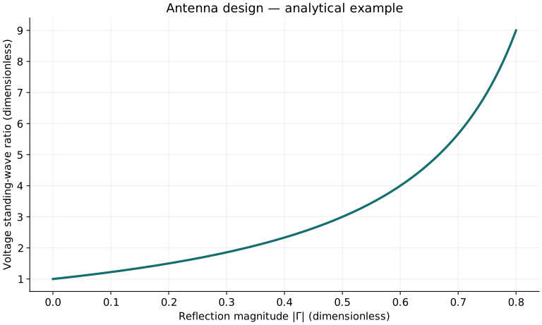
Twenty worked examples
Open a problem to see its defined inputs, assumptions, equation, numerical substitution, result, and interpretation. Values are illustrative analytical exercises.
Example 01. Free-space wavelength
Definitions & inputs. f=1 GHz, c=299792458 m/s.
Choose the governing model and isolate the requested quantity.
Insert the stated inputs in consistent units or the explicitly defined normalized units.
Evaluate the expression; the result uses the units shown.
Interpretation. Wavelength in a dielectric differs from the free-space value.
↑ Return to definitions and contentsExample 02. Nominal half-wave dipole
Definitions & inputs. f=100 MHz in free space.
Choose the governing model and isolate the requested quantity.
Insert the stated inputs in consistent units or the explicitly defined normalized units.
Evaluate the expression; the result uses the units shown.
Interpretation. Resonant physical length is affected by radius, end effects, and mounting.
↑ Return to definitions and contentsExample 03. Nominal quarter-wave monopole
Definitions & inputs. f=300 MHz over an ideal infinite ground plane.
Choose the governing model and isolate the requested quantity.
Insert the stated inputs in consistent units or the explicitly defined normalized units.
Evaluate the expression; the result uses the units shown.
Interpretation. A finite ground plane changes pattern and resonance.
↑ Return to definitions and contentsExample 04. Gain from efficiency
Definitions & inputs. Directivity 8, radiation efficiency .75.
Choose the governing model and isolate the requested quantity.
Insert the stated inputs in consistent units or the explicitly defined normalized units.
Evaluate the expression; the result uses the units shown.
Interpretation. This gain excludes impedance mismatch.
↑ Return to definitions and contentsExample 05. Gain in dBi
Definitions & inputs. Linear gain 6.
Choose the governing model and isolate the requested quantity.
Insert the stated inputs in consistent units or the explicitly defined normalized units.
Evaluate the expression; the result uses the units shown.
Interpretation. Isotropic gain is the reference.
↑ Return to definitions and contentsExample 06. Reflection coefficient
Definitions & inputs. Real antenna resistance 75 Ω on 50 Ω line.
Choose the governing model and isolate the requested quantity.
Insert the stated inputs in consistent units or the explicitly defined normalized units.
Evaluate the expression; the result uses the units shown.
Interpretation. The reflection phase is zero in this resistive example.
↑ Return to definitions and contentsExample 07. VSWR
Definitions & inputs. Reflection magnitude .2.
Choose the governing model and isolate the requested quantity.
Insert the stated inputs in consistent units or the explicitly defined normalized units.
Evaluate the expression; the result uses the units shown.
Interpretation. A ratio of one indicates perfect impedance match.
↑ Return to definitions and contentsExample 08. Return loss
Definitions & inputs. Reflection magnitude .2.
Choose the governing model and isolate the requested quantity.
Insert the stated inputs in consistent units or the explicitly defined normalized units.
Evaluate the expression; the result uses the units shown.
Interpretation. Larger return loss means less reflection.
↑ Return to definitions and contentsExample 09. Mismatch efficiency
Definitions & inputs. Reflection magnitude .2.
Choose the governing model and isolate the requested quantity.
Insert the stated inputs in consistent units or the explicitly defined normalized units.
Evaluate the expression; the result uses the units shown.
Interpretation. Four percent of incident power reflects at this interface.
↑ Return to definitions and contentsExample 10. Radiation efficiency
Definitions & inputs. Radiation resistance 60 Ω, loss resistance 15 Ω.
Choose the governing model and isolate the requested quantity.
Insert the stated inputs in consistent units or the explicitly defined normalized units.
Evaluate the expression; the result uses the units shown.
Interpretation. Both resistances use the same feed-current convention.
↑ Return to definitions and contentsExample 11. Short-dipole resistance
Definitions & inputs. Triangular-current short dipole, total length L=.05λ.
Choose the governing model and isolate the requested quantity.
Insert the stated inputs in consistent units or the explicitly defined normalized units.
Evaluate the expression; the result uses the units shown.
Interpretation. The uniform-current Hertzian dipole has a different coefficient.
↑ Return to definitions and contentsExample 12. Effective aperture
Definitions & inputs. Gain 10, wavelength .1 m.
Choose the governing model and isolate the requested quantity.
Insert the stated inputs in consistent units or the explicitly defined normalized units.
Evaluate the expression; the result uses the units shown.
Interpretation. Receiving polarization and impedance are matched.
↑ Return to definitions and contentsExample 13. Dish gain
Definitions & inputs. Diameter 1 m, wavelength .03 m, aperture efficiency .6.
Choose the governing model and isolate the requested quantity.
Insert the stated inputs in consistent units or the explicitly defined normalized units.
Evaluate the expression; the result uses the units shown.
Interpretation. Aperture efficiency includes illumination and other aperture losses.
↑ Return to definitions and contentsExample 14. Dish approximate beamwidth
Definitions & inputs. D=1 m, λ=.03 m; illustrative 70° coefficient.
Choose the governing model and isolate the requested quantity.
Insert the stated inputs in consistent units or the explicitly defined normalized units.
Evaluate the expression; the result uses the units shown.
Interpretation. The coefficient depends on illumination; this is not a universal dish specification.
↑ Return to definitions and contentsExample 15. Far-field distance estimate
Definitions & inputs. Aperture maximum size 1 m, λ=.03 m.
Choose the governing model and isolate the requested quantity.
Insert the stated inputs in consistent units or the explicitly defined normalized units.
Evaluate the expression; the result uses the units shown.
Interpretation. Also require distance large compared with wavelength and antenna dimensions.
↑ Return to definitions and contentsExample 16. Isotropic power density
Definitions & inputs. Radiated power 10 W, distance 100 m.
Choose the governing model and isolate the requested quantity.
Insert the stated inputs in consistent units or the explicitly defined normalized units.
Evaluate the expression; the result uses the units shown.
Interpretation. The isotropic source is a normalization model.
↑ Return to definitions and contentsExample 17. EIRP
Definitions & inputs. Transmit accepted power 2 W, transmit gain 10.
Choose the governing model and isolate the requested quantity.
Insert the stated inputs in consistent units or the explicitly defined normalized units.
Evaluate the expression; the result uses the units shown.
Interpretation. Feed cable loss must be applied before accepted antenna power.
↑ Return to definitions and contentsExample 18. Friis received power
Definitions & inputs. Pt=1 W, Gt=Gr=1, λ=.1 m, r=100 m.
Choose the governing model and isolate the requested quantity.
Insert the stated inputs in consistent units or the explicitly defined normalized units.
Evaluate the expression; the result uses the units shown.
Interpretation. This is a matched, unobstructed free-space link.
↑ Return to definitions and contentsExample 19. Polarization coupling
Definitions & inputs. Two linear polarizations separated by 30°.
Choose the governing model and isolate the requested quantity.
Insert the stated inputs in consistent units or the explicitly defined normalized units.
Evaluate the expression; the result uses the units shown.
Interpretation. Circular/elliptical states need a vector polarization calculation.
↑ Return to definitions and contentsExample 20. Array steering phase
Definitions & inputs. Half-wavelength element spacing, beam θ0=30° from broadside.
Choose the governing model and isolate the requested quantity.
Insert the stated inputs in consistent units or the explicitly defined normalized units.
Evaluate the expression; the result uses the units shown.
Interpretation. Adjacent element phase is negative under the stated array convention.
↑ Return to definitions and contentsSymbols and units
Each derivation and problem defines its own symbols and inputs. Symbols may be reused with different meanings in other subjects. Keep units consistent, retain sufficient precision during calculation, and apply the stated validity limits.