PHYSICS / ENGINEERING / COMPUTING
Atomic physics: bound states, spectra and interactions
Use quantum mechanics to derive atomic structure and spectra, then connect interacting atoms to solids, liquids, gases and plasmas.
Matter pathway: atom → solid → liquid → gas → plasma. Quantum mechanics and quantum field theory provide foundations across the pathway; they are not additional phases. This is a connected modeling route, not a universal heating curve. Actual phases depend on pressure, composition, and kinetics.
1. Coulomb bound states
Definitions & inputs. μ reduced electron–nucleus mass,Z nuclear charge,n principal quantum number,l orbital quantum number,m its projection.
Separate relative motion from center-of-mass motion.
Spherical symmetry separates the radial and angular equations; normalizability quantizes the radial solution.
Requiring the radial series to terminate yields the discrete energy spectrum.
Interpretation. Quantum orbitals are probability amplitudes, not classical planetary trajectories.
↑ Return to definitions and contents2. Spectra and dipole transitions
Definitions & inputs. ν photon frequency,λ wavelength,d electric dipole operator.
Energy conservation relates a downward level transition to emitted light.
Transition strength depends on a matrix element, not merely an energy difference.
Angular parity and the vector operator give electric-dipole selection rules in the orbital basis.
Interpretation. Spin, total angular momentum and coupling scheme add selection rules; forbidden dipole transitions may occur through higher multipoles or multiple photons.
↑ Return to definitions and contents3. Many-electron atoms and external fields
Definitions & inputs. H electron Hamiltonian,rij electron separation,μB Bohr magneton,gJ Landé factor,mJ angular projection.
Electron–electron repulsion prevents the simple hydrogenic separation.
Antisymmetry enforces fermionic exchange and Pauli exclusion; use spin orbitals.
First-order perturbation in a weak magnetic field splits angular-momentum states.
Interpretation. Hartree–Fock, configuration interaction and density functional methods offer different approximations; screening with an effective Z is only a rough model.
↑ Return to definitions and contents4. From isolated atoms to matter
Definitions & inputs. R internuclear spacing,t hopping energy,k wavevector,a lattice spacing,ne electron density.
Overlapping atomic orbitals form a many-site electronic model.
Fourier-transform a one-dimensional periodic chain to obtain a band from one atomic level.
When atoms ionize into a suitable weakly coupled plasma, collective screening introduces a different length scale.
Interpretation. Solids have ordered or disordered bonded structure; liquids have persistent short-range correlations; gases may have atoms or molecules; plasmas add free charges. Quantum foundations apply throughout, not just at the atomic stage.
↑ Return to definitions and contentsGraphical worked example
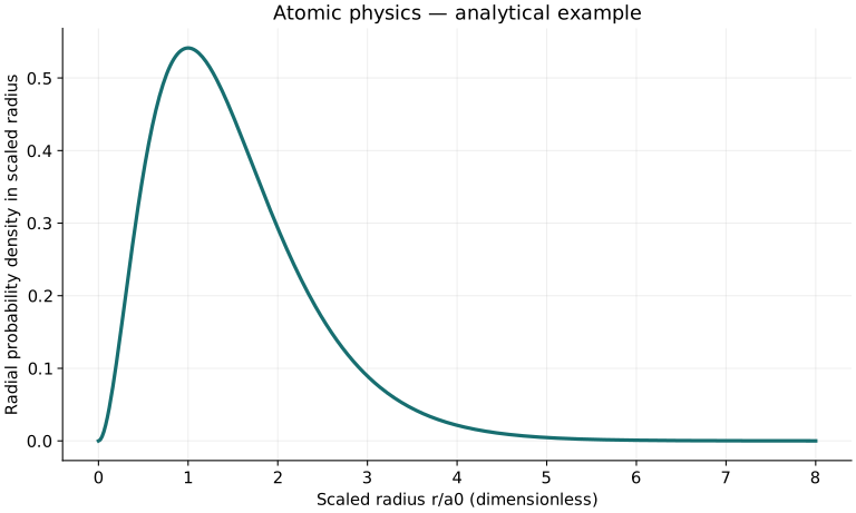
Twenty worked examples
Open a problem to see its defined inputs, assumptions, equation, numerical substitution, result, and interpretation. Values are illustrative analytical exercises.
Example 01. Hydrogen ground energy
Definitions & inputs. Z1,n1.
Choose the governing model and isolate the requested quantity.
Insert the stated inputs in consistent units or the explicitly defined normalized units.
Evaluate the expression; the result uses the units shown.
Interpretation. Rounded infinite-mass Coulomb benchmark.
↑ Return to definitions and contentsExample 02. Hydrogen second level
Definitions & inputs. Z1,n2.
Choose the governing model and isolate the requested quantity.
Insert the stated inputs in consistent units or the explicitly defined normalized units.
Evaluate the expression; the result uses the units shown.
Interpretation. Excludes fine structure.
↑ Return to definitions and contentsExample 03. Hydrogen third level
Definitions & inputs. n3.
Choose the governing model and isolate the requested quantity.
Insert the stated inputs in consistent units or the explicitly defined normalized units.
Evaluate the expression; the result uses the units shown.
Interpretation. Single-electron approximation.
↑ Return to definitions and contentsExample 04. Ground ionization energy
Definitions & inputs. E1=−13.6eV,continuum0.
Choose the governing model and isolate the requested quantity.
Insert the stated inputs in consistent units or the explicitly defined normalized units.
Evaluate the expression; the result uses the units shown.
Interpretation. Ionization removes the electron to zero kinetic energy at infinity.
↑ Return to definitions and contentsExample 05. Excited-state ionization
Definitions & inputs. n2.
Choose the governing model and isolate the requested quantity.
Insert the stated inputs in consistent units or the explicitly defined normalized units.
Evaluate the expression; the result uses the units shown.
Interpretation. Smaller binding at largern.
↑ Return to definitions and contentsExample 06. Lyman-alpha energy
Definitions & inputs. Transition2→1.
Choose the governing model and isolate the requested quantity.
Insert the stated inputs in consistent units or the explicitly defined normalized units.
Evaluate the expression; the result uses the units shown.
Interpretation. Actual allowed2p→1s transition.
↑ Return to definitions and contentsExample 07. Lyman-alpha wavelength
Definitions & inputs. Photon10.2eV.
Choose the governing model and isolate the requested quantity.
Insert the stated inputs in consistent units or the explicitly defined normalized units.
Evaluate the expression; the result uses the units shown.
Interpretation. Rounded model, not a precision reference wavelength.
↑ Return to definitions and contentsExample 08. Balmer-alpha energy
Definitions & inputs. 3→2.
Choose the governing model and isolate the requested quantity.
Insert the stated inputs in consistent units or the explicitly defined normalized units.
Evaluate the expression; the result uses the units shown.
Interpretation. Allowed orbital sublevels must also be chosen.
↑ Return to definitions and contentsExample 09. Balmer-alpha wavelength
Definitions & inputs. Same photon.
Choose the governing model and isolate the requested quantity.
Insert the stated inputs in consistent units or the explicitly defined normalized units.
Evaluate the expression; the result uses the units shown.
Interpretation. Vacuum model wavelength.
↑ Return to definitions and contentsExample 10. Hydrogenic helium energy
Definitions & inputs. HeplusZ2,n1.
Choose the governing model and isolate the requested quantity.
Insert the stated inputs in consistent units or the explicitly defined normalized units.
Evaluate the expression; the result uses the units shown.
Interpretation. Does not describe neutral helium.
↑ Return to definitions and contentsExample 11. Most-probable1s radius
Definitions & inputs. Z2,a0=.0529177nm.
Choose the governing model and isolate the requested quantity.
Insert the stated inputs in consistent units or the explicitly defined normalized units.
Evaluate the expression; the result uses the units shown.
Interpretation. Peak of the radial probability distribution.
↑ Return to definitions and contentsExample 12. Mean1s radius
Definitions & inputs. Hydrogen a0=.0529177nm.
Choose the governing model and isolate the requested quantity.
Insert the stated inputs in consistent units or the explicitly defined normalized units.
Evaluate the expression; the result uses the units shown.
Interpretation. Differs from most-probable radius.
↑ Return to definitions and contentsExample 13. Orbital degeneracy
Definitions & inputs. Principal n3,ignore spin.
Choose the governing model and isolate the requested quantity.
Insert the stated inputs in consistent units or the explicitly defined normalized units.
Evaluate the expression; the result uses the units shown.
Interpretation. Coulomb degeneracy before perturbations.
↑ Return to definitions and contentsExample 14. Shell capacity
Definitions & inputs. n3,including two spin states.
Choose the governing model and isolate the requested quantity.
Insert the stated inputs in consistent units or the explicitly defined normalized units.
Evaluate the expression; the result uses the units shown.
Interpretation. Pauli spin-orbital count.
↑ Return to definitions and contentsExample 15. Angular momentum magnitude
Definitions & inputs. l1.
Choose the governing model and isolate the requested quantity.
Insert the stated inputs in consistent units or the explicitly defined normalized units.
Evaluate the expression; the result uses the units shown.
Interpretation. Magnitude differs from maximal projection.
↑ Return to definitions and contentsExample 16. Weak Zeeman shift
Definitions & inputs. μB5.7883818×10⁻⁵eV/T,gJ2,mJ.5,B1T.
Choose the governing model and isolate the requested quantity.
Insert the stated inputs in consistent units or the explicitly defined normalized units.
Evaluate the expression; the result uses the units shown.
Interpretation. Weak-field perturbative example.
↑ Return to definitions and contentsExample 17. Natural lifetime scale
Definitions & inputs. DecayA10⁸/s.
Choose the governing model and isolate the requested quantity.
Insert the stated inputs in consistent units or the explicitly defined normalized units.
Evaluate the expression; the result uses the units shown.
Interpretation. One dominant spontaneous channel.
↑ Return to definitions and contentsExample 18. Lifetime-limited linewidth
Definitions & inputs. τ10ns.
Choose the governing model and isolate the requested quantity.
Insert the stated inputs in consistent units or the explicitly defined normalized units.
Evaluate the expression; the result uses the units shown.
Interpretation. Lorentzian FWHM for exponential population decay without extra dephasing.
↑ Return to definitions and contentsExample 19. Thermal population ratio
Definitions & inputs. Equal degeneracies,ΔE1eV,kBT.5eV.
Choose the governing model and isolate the requested quantity.
Insert the stated inputs in consistent units or the explicitly defined normalized units.
Evaluate the expression; the result uses the units shown.
Interpretation. Thermal equilibrium; not arbitrary laser-driven populations.
↑ Return to definitions and contentsExample 20. Atomic-level band width
Definitions & inputs. 1D nearest-neighbor t1eV.
Choose the governing model and isolate the requested quantity.
Insert the stated inputs in consistent units or the explicitly defined normalized units.
Evaluate the expression; the result uses the units shown.
Interpretation. One-orbital tight-binding chain.
↑ Return to definitions and contentsSymbols and units
Each derivation and problem defines its own symbols and inputs. Symbols may be reused with different meanings in other subjects. Keep units consistent, retain sufficient precision during calculation, and apply the stated validity limits.