Liquid-state physics

1. Definitions: g(r) counts neighbors; h(r) measures the excess

Definitions & inputs. N is particle count, V volume, n=N/V number density (m⁻³), r a separation (m), and k a wavevector magnitude (m⁻¹). g(r), h(r), c(r), and S(k) are dimensionless. Their three-dimensional Fourier transforms have units of volume. Here g(r) is a pair distribution, not Gibbs energy; h(r) is a total correlation, not enthalpy or Planck’s constant.

1. The two-particle density n^(2) counts distinct-particle pairs per product of volume elements. Divide by n² to define the radial pair distribution.

   $$n^{(2)}(\mathbf r_1,\mathbf r_2)=n^2g(r),\qquad r=|\mathbf r_1-\mathbf r_2|$$

2. Conditional on one tagged particle, dz is the mean number of other particles in a shell. g alone is neither a shell count nor a probability density normalized to one.

   $$dz=4\pi n r^2g(r)\,dr$$

3. Subtract the uncorrelated baseline g=1. Positive h indicates an excess of neighbors at that separation; negative h indicates depletion.

   $$h(r)=g(r)-1,\qquad dz-dz_{\mathrm{uncorrelated}}=4\pi nr^2h(r)\,dr$$

4. Examples: a peak need not be bounded by one; an excluded hard core has g=0. Since g is nonnegative, h cannot be smaller than −1.

   $$g=2.5\Rightarrow h=1.5,\qquad g=0.2\Rightarrow h=-0.8,\qquad g=0\Rightarrow h=-1$$

Interpretation. For a uniform ordinary fluid far from criticality, g tends to one and h tends to zero at large separation. The coordination number is an integral of g over a chosen shell, not the peak height.

• Schirmacher — Theory of liquids and polymers ↗

2. Worked example: count a shell of neighbors

Definitions & inputs. Take n=0.05 Å⁻³ and approximate g(r)=2 throughout the shell 2 Å≤r≤3 Å. z is the mean neighbor count, not an integer for every configuration.

1. Start with the conditional shell count and integrate over the shell.

   $$z=4\pi n\int_{r_1}^{r_2}r^2g(r)\,dr$$

2. The ų from the integral cancels Å⁻³ from density.

   $$z=4\pi(0.05)(2)\left[\frac{r^3}{3}\right]_2^3=\frac{0.4\pi}{3}(27-8)=7.95870$$

3. With h=1 in the shell, the excess count equals the uncorrelated baseline.

   $$z_{g=1}=3.97935,\qquad\Delta z=4\pi n\int_2^3r^2h(r)\,dr=3.97935$$

Interpretation. A peak height of two means twice the local density; here the finite shell contains about eight neighbors on average.

• Schirmacher — Theory of liquids and polymers ↗

3. Derive S(k): real-space correlations become density fluctuations

Definitions & inputs. ρk=Σj exp(−ik·rj) is a microscopic number-density mode, not mass density. δρk=ρk−⟨ρk⟩ removes the mean. Angular brackets denote an ensemble average. S(k) is the static number-number structure factor.

1. Define the nonnegative fluctuation power per particle. For nonzero k in a uniform bulk fluid, the mean Fourier mode vanishes.

   $$S(k)=\frac{\langle\delta\rho_{\mathbf k}\delta\rho_{-\mathbf k}\rangle}{\langle N\rangle},\qquad\rho_{\mathbf k}=\sum_j e^{-i\mathbf k\cdot\mathbf r_j}$$

2. Expand the double particle sum. Terms with the same particle give the self contribution 1; distinct-particle excess correlations give n times the transform of h.

   $$S(k)=1+n\widehat h(k),\qquad\widehat h(\mathbf k)=\int h(r)e^{-i\mathbf k\cdot\mathbf r}\,d^3r$$

3. Choose the polar axis parallel to k and substitute μ=cos θ. Here μ is only an angular integration variable, not the chemical potential used later. This step explains the spherical transform kernel.

   $$\int e^{-ikr\cos\theta}d\Omega=2\pi\int_{-1}^{1}e^{-ikr\mu}d\mu=4\pi\frac{\sin(kr)}{kr}$$

4. Perform the angular integral for an isotropic fluid. The factor sin(kr)/(kr) weights different separations with alternating signs; S is not simply g with its axis relabeled.

   $$S(k)=1+4\pi n\int_0^\infty h(r)\frac{\sin(kr)}{kr}r^2\,dr$$

5. This inverse uses the stated Fourier convention, with (2π)⁻³ in the inverse three-dimensional transform. Finite measured k ranges introduce resolution and truncation errors.

   $$h(r)=\frac{1}{2\pi^2n}\int_0^\infty[S(k)-1]\frac{\sin(kr)}{kr}k^2\,dk$$

6. Take the long-wavelength limit, using sin(kr)/(kr)→1 when the correlation integral converges. It probes large-scale density fluctuations, not just the first shell.

   $$S(0^+)=1+4\pi n\int_0^\infty h(r)r^2\,dr$$

Interpretation. In a fixed-N simulation, the exactly zero connected mode is zero because N cannot fluctuate. Compressibility uses the bulk k→0 limit, not that finite-box k=0 bin. For integrable h, S(k) approaches one at large k. A peak in S identifies a prominent correlation length, not a phase or pressure by itself.

• Schirmacher — Theory of liquids and polymers ↗

4. Compare gas, liquid, and solid structure

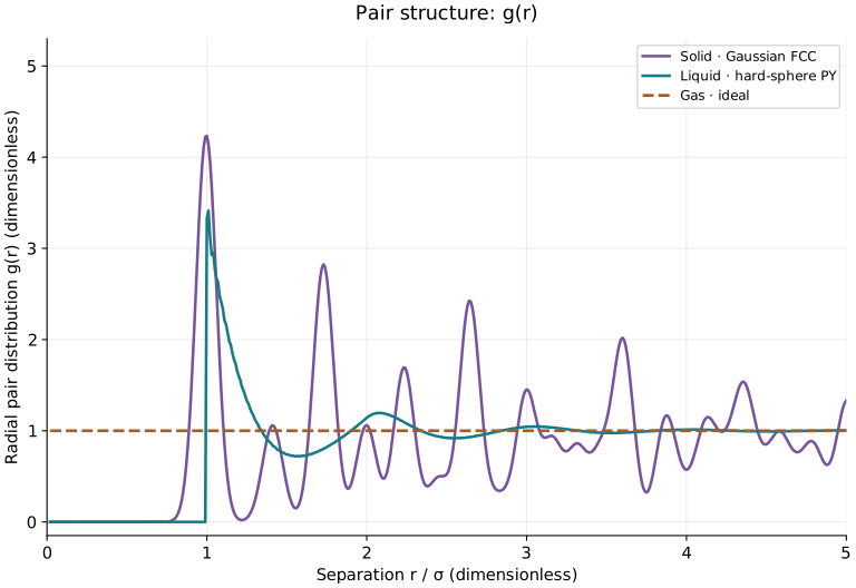
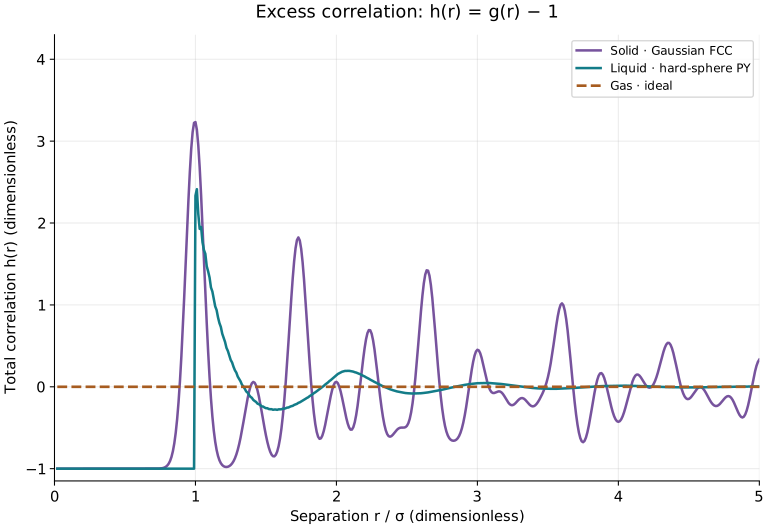
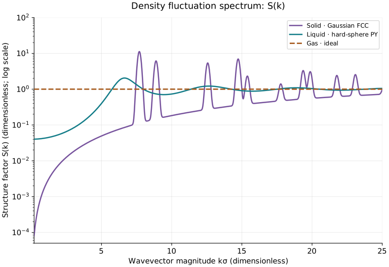
The same colors identify each reference model in all three plots. σ is a reference length: the liquid hard-sphere diameter and the solid nearest-neighbor lattice spacing. All functions are dimensionless; S(k) uses a logarithmic vertical axis so both low-k suppression and sharp peaks remain visible.

Reproducible plot data: g(r) and h(r) CSV · S(k) CSV · All data and parameters (JSON)

5. Separate total, direct, and indirect correlations

Definitions & inputs. c(r) is the direct correlation defined through Ornstein-Zernike (OZ). γ(r)=h(r)−c(r) is the indirect correlation. Thus h is total, c direct, and γ indirect. β=1/(kBT); u(r) is a pair interaction energy, not a displacement or flow velocity.

1. OZ separates a direct part from a convolution representing correlations mediated through other particles. c is not generally equal to the force or pair potential.

   $$h(r)=c(r)+n\int c(|\mathbf r-\mathbf r^{\prime}|)h(r^{\prime})\,d^3r^{\prime}$$

2. A Fourier transform converts the convolution into multiplication. Rearrange to solve algebraically for the total correlation transform.

   $$\widehat h=\widehat c+n\widehat c\widehat h\quad\Rightarrow\quad\widehat h=\frac{\widehat c}{1-n\widehat c}$$

3. Move the indirect term to the left and factor out h-hat. To obtain S, put the self contribution one over the same denominator; the two terms containing n c-hat in the numerator cancel.

   $$(1-n\widehat c)\widehat h=\widehat c,\qquad 1+n\widehat h=\frac{1-n\widehat c+n\widehat c}{1-n\widehat c}$$

4. Substitute into the structure-factor identity. The number-density factor is required for dimensional consistency.

   $$S(k)=1+n\widehat h(k)=\frac{1}{1-n\widehat c(k)}$$

5. HNC and PY close OZ differently. They are approximations to many-particle structure, not interchangeable definitions of g.

   $$\gamma=h-c,\qquad g_{\mathrm{HNC}}=e^{-\beta u+\gamma},\qquad g_{\mathrm{PY}}=e^{-\beta u}(1+\gamma)$$

Interpretation. The often useful approximation c≈−βu is a further closure in restricted regimes; it is not the definition of direct correlation. An approximate closure may predict different pressures through different thermodynamic routes.

• Schirmacher — Theory of liquids and polymers ↗

6. Close OZ and solve it numerically

Definitions & inputs. γ=h−c is the indirect correlation; b(r)=exp[−βu(r)] is the Boltzmann factor; Bbr is the bridge function collecting correlations omitted by HNC. Superscript m labels an iteration, α is a mixing parameter, and ε is a residual tolerance.

1. The exact formal closure introduces an unknown bridge function. HNC neglects it; OZ alone has two unknown functions and is not closed.

   $$g=e^{-\beta u+\gamma+B_{\rm br}},\qquad B_{\rm br}=0\ \Rightarrow\ g_{\rm HNC}=b e^\gamma$$

2. PY uses a different approximation. Replacing e^γ by 1+γ in HNC is a useful algebraic comparison, not an exact derivation of PY at arbitrary density; the full Boltzmann factor is retained.

   $$g_{\rm PY}=b(1+\gamma),\qquad c_{\rm PY}=(b-1)(1+\gamma)$$

3. Specify u,n,T, choose a radial grid and cutoff, then compute c from the current γ. Begin at low density if necessary.

   $$\gamma^{(0)}=0;\quad c^{(m)}_{\rm HNC}=b e^{\gamma^{(m)}}-1-\gamma^{(m)},\quad c^{(m)}_{\rm PY}=(b-1)(1+\gamma^{(m)})$$

4. Apply the spherical Fourier transform and use γ-hat=h-hat−c-hat. An ordinary one-dimensional FFT of c is not this transform.

   $$\widehat c(k)=4\pi\int_0^\infty c(r)\frac{\sin kr}{kr}r^2dr,\qquad \widehat\gamma_{\rm trial}(k)=\frac{n\widehat c(k)^2}{1-n\widehat c(k)}$$

5. Invert with the matching normalization. Treat r=0 and k=0 with their analytic sinc limits.

   $$\gamma_{\rm trial}(r)=\frac1{2\pi^2}\int_0^\infty\widehat\gamma_{\rm trial}(k)\frac{\sin kr}{kr}k^2dk$$

6. Check the unmixed residual Rm, then damp the update, for example α=0.1. Stop only after the residual is below the chosen tolerance; small damping alone must not falsely signal convergence.

   $$R_m=\max_r|\gamma_{\rm trial}-\gamma^{(m)}|,\quad\gamma^{(m+1)}=(1-\alpha)\gamma^{(m)}+\alpha\gamma_{\rm trial},\quad0<\alpha\leq1$$

7. For a hard core, enforce the last identities directly and avoid log(g). Check g≥0 and S≥0, refine the mesh and cutoff, and compare pressure routes.

   $$g=1+c+\gamma,\quad S=(1-n\widehat c)^{-1};\qquad r<\sigma:\ b=0,\ g=0,\ c=-1-\gamma$$

Interpretation. Repeat closure → transform → OZ → inverse transform → mixing. Use density continuation or a more robust nonlinear solver if the iteration fails. This is an algorithm lesson, not a claim that a full liquid solver runs in this page.

• Schirmacher — Theory of liquids and polymers ↗

7. Worked example: one local closure and mixing step

Definitions & inputs. At one radial grid point outside a core, let βu=0.5, γ=0.2. For a separate iteration illustration let γtrial=0.35 and α=0.1.

1. Compute the Boltzmann factor and the HNC pair value.

   $$b=e^{-0.5}=0.606531,\qquad g_{\rm HNC}=e^{-0.5+0.2}=0.740818$$

2. Subtract the uncorrelated baseline and indirect correlation.

   $$c_{\rm HNC}=g-1-\gamma=0.740818-1-0.2=-0.459182$$

3. Use the same potential and indirect correlation to compare PY with HNC.

   $$g_{\rm PY}=0.606531(1.2)=0.727837,\quad c_{\rm PY}=0.727837-1.2=-0.472163$$

4. Damping changes the iterate by only 0.015, but the unmixed local residual is ten times larger.

   $$R_{\rm local}=|0.35-0.20|=0.15,\qquad\gamma_{\rm next}=0.9(0.20)+0.1(0.35)=0.215$$

Interpretation. The closures agree to first order in small γ, but differ at finite γ. A small update caused by damping is not evidence of a small equation residual.

• Schirmacher — Theory of liquids and polymers ↗

8. Pressure route A: weight g(r) by the pair force

Definitions & inputs. p is pressure (Pa); u′(r)=du/dr; the central pair force is −u′(r) r-hat. Z=p/(nkBT) is the compressibility factor, distinct from both a partition function and the structure factor S(k).

1. The mechanical virial adds the interaction contribution to the kinetic ideal-gas pressure.

   $$pV=Nk_{\mathrm B}T+\frac13\left\langle\sum_{i<j}\mathbf r_{ij}\cdot\mathbf F_{ij}\right\rangle$$

2. For a central force, reduce the vector dot product to a radial derivative.

   $$\mathbf r_{ij}\cdot\mathbf F_{ij}=-r_{ij}u^{\prime}(r_{ij})$$

3. Use pair statistics to replace the distinct unordered-pair sum. The factor one half avoids counting each pair twice.

   $$\frac1V\left\langle\sum_{i<j}A(r_{ij})\right\rangle=\frac{n^2}{2}\int A(r)g(r)\,d^3r$$

4. Insert A=−ru′ and the spherical volume element 4πr²dr. This is the virial pressure route.

   $$p=nk_{\mathrm B}T-\frac{2\pi n^2}{3}\int_0^\infty r^3u^{\prime}(r)g(r)\,dr$$

5. Express the same result in terms of excess correlations. Simply knowing a peak in g or h is insufficient: pressure depends on the force-weighted integral over all separations.

   $$g=1+h\quad\Rightarrow\quad p=nk_{\mathrm B}T-\frac{2\pi n^2}{3}\int_0^\infty r^3u^{\prime}(r)[1+h(r)]\,dr$$

Interpretation. Where u′<0, a repulsive pair-force contribution raises pressure; where u′>0, an attractive contribution lowers it. The sum determines the result. Hard spheres have a discontinuous potential and must use a contact relation instead of ordinary differentiation.

• Schirmacher — Theory of liquids and polymers ↗

9. Pressure route B: use S(0) to obtain the isothermal slope

Definitions & inputs. κT=−(1/V)(∂V/∂p)T,N is isothermal compressibility (Pa⁻¹), measuring how readily density changes under pressure. KT=1/κT is the bulk modulus. S(0+) is the bulk long-wavelength limit, and μ is chemical potential per particle.

1. Differentiate grand-canonical averages with respect to chemical potential: the number response is proportional to the number variance.

   $$\langle(\Delta N)^2\rangle=k_{\mathrm B}T\left(\frac{\partial\langle N\rangle}{\partial\mu}\right)_{T,V}$$

2. Use Gibbs-Duhem at fixed temperature and the definition of compressibility.

   $$dp=n\,d\mu\quad(T\ \mathrm{fixed}),\qquad\left(\frac{\partial n}{\partial p}\right)_T=n\kappa_T$$

3. Combine the two responses. Smaller S(0+) means weaker long-wavelength fluctuations and a larger bulk modulus at the same n,T.

   $$S(0^+)=\frac{\langle(\Delta N)^2\rangle}{\langle N\rangle}=nk_{\mathrm B}T\kappa_T$$

4. Invert the density response. S at one state gives a pressure derivative, not an absolute pressure.

   $$\left(\frac{\partial p}{\partial n}\right)_T=\frac{k_{\mathrm B}T}{S(0^+;n,T)}$$

5. Integrate along a specified single-phase isotherm and supply a reference pressure. Integrating from vacuum with p(0)=0 is only justified if the required branch is valid and connected.

   $$p(n,T)=p(n_{\mathrm{ref}},T)+k_{\mathrm B}T\int_{n_{\mathrm{ref}}}^{n}\frac{dn^{\prime}}{S(0^+;n^{\prime},T)}$$

6. Differentiate p=nkBT Z. In general S(0+) is NOT 1/Z; the density dependence of Z supplies an extra term.

   $$\frac1{S(0^+)}=Z+n\left(\frac{\partial Z}{\partial n}\right)_T$$

Interpretation. Exact equilibrium correlations and consistent interactions give agreement between pressure routes. Approximate PY/HNC closures may be thermodynamically inconsistent. Finite-size effects, correlation tails, and noisy low-k data can strongly affect compressibility estimates.

• Schirmacher — Theory of liquids and polymers ↗

10. Worked example: scattering to compressibility and bulk modulus

Definitions & inputs. Use n=2.5×10²⁸ m⁻³, T=300 K, S(0+)=0.050, and kB=1.380649×10⁻²³ J K⁻¹. KT is the isothermal bulk modulus.

1. Calculate the ideal pressure scale; joules per cubic metre are pascals.

   $$nk_{\rm B}T=(2.5\times10^{28})(1.380649\times10^{-23})(300)=1.03548675\times10^8\ {\rm Pa}$$

2. Divide the dimensionless fluctuation level by the pressure scale.

   $$\kappa_T=\frac{S(0^+)}{nk_{\rm B}T}=4.82865\times10^{-10}\ {\rm Pa}^{-1}$$

3. Invert the compressibility to obtain the bulk modulus.

   $$K_T=\kappa_T^{-1}=2.0709735\times10^9\ {\rm Pa}=2.07097\ {\rm GPa}$$

4. A small isothermal pressure increase of 1 MPa produces approximately a 0.0483% density increase if κ is locally constant.

   $$\frac{\Delta n}{n}\simeq\kappa_T\Delta p=(4.82865\times10^{-10})(10^6)=4.82865\times10^{-4}$$

Interpretation. These inputs determine a local stiffness, not an absolute pressure. Recovering p requires an isothermal density path and reference pressure.

• Schirmacher — Theory of liquids and polymers ↗

11. Energy route: pair counting and the missing free-energy reference

Definitions & inputs. E is total internal energy, Uex the mean pair interaction energy, Fex the excess Helmholtz free energy, and fex=Fex/N. u is a temperature-independent pair energy.

1. Equipartition gives the kinetic contribution; unordered pairs contribute interaction energy.

   $$\frac{E}{N}=\frac32k_{\rm B}T+\frac1N\left\langle\sum_{i<j}u(r_{ij})\right\rangle$$

2. Replace the pair sum by its pair-density integral; the one-half removes double counting.

   $$\frac{U_{\rm ex}}N=\frac n2\int u(r)g(r)d^3r=2\pi n\int_0^\infty u(r)g(r)r^2dr$$

3. Integrate energy at fixed density to obtain free energy only after supplying a consistent reference.

   $$\left(\frac{\partial(\beta f_{\rm ex})}{\partial\beta}\right)_n=\frac{U_{\rm ex}}N,\quad \beta f_{\rm ex}(\beta,n)=\beta_0 f_{\rm ex}(\beta_0,n)+\int_{\beta_0}^{\beta}\frac{U_{\rm ex}(\beta^\prime,n)}N d\beta^\prime$$

4. Differentiate free energy with respect to density to obtain pressure. An energy at a single state is insufficient.

   $$p=nk_{\rm B}T+n^2\left(\frac{\partial f_{\rm ex}}{\partial n}\right)_T$$

5. Allowed hard-sphere configurations have zero potential energy; overlapping configurations are forbidden. Do not assign a value to infinity times zero. The excess free energy is entropic and still density-dependent.

   $$\text{Hard spheres:}\quad U_{\rm ex}=0,\quad E/N=\tfrac32 k_{\rm B}T,\quad p\ne nk_{\rm B}T\ \ (n>0)$$

Interpretation. A hard-sphere energy alone cannot recover its nonideal pressure: the density-dependent entropic reference is essential.

• Schirmacher — Theory of liquids and polymers ↗

12. Worked example: attractive-shell interaction energy

Definitions & inputs. A hard core has diameter σ; outside it u=−ε for σ<r<λσ and zero beyond λσ. Approximate g=g0 in this attractive shell. Choose nσ³=0.1, λ=1.5, g0=1, ε=kBT.

1. Only the allowed attractive shell contributes potential energy.

   $$\frac{U_{\rm ex}}N=2\pi n\int_\sigma^{\lambda\sigma}(-\epsilon)g_0r^2dr$$

2. Integrate r² to r³/3; dividing by ε makes the result dimensionless.

   $$\frac{U_{\rm ex}}{N\epsilon}=-\frac{2\pi}{3}(n\sigma^3)g_0(\lambda^3-1)$$

3. Insert the specified reduced density and well width.

   $$\frac{U_{\rm ex}}{N\epsilon}=-\frac{2\pi}{3}(0.1)(3.375-1)=-0.497419$$

4. Add translational kinetic energy, using ε=kBT at the stated temperature.

   $$\frac E{Nk_{\rm B}T}=\frac32-0.497419=1.002581$$

Interpretation. Attraction lowers energy. This single-state estimate does not supply the temperature dependence or reference needed to derive an equation of state.

• Schirmacher — Theory of liquids and polymers ↗

13. Hard spheres: derive the two PY pressures and Carnahan–Starling

Definitions & inputs. σ is sphere diameter; φ=πnσ³/6 is packing fraction; g(σ+) is the right-hand contact value. Zv and Zc denote virial and compressibility-route p/(nkBT). y=g/exp(−βu) is the cavity function defined by a smooth-core limit.

1. Take the steep repulsion limit in the Boltzmann factor. This avoids differentiating an infinite potential or multiplying infinity by zero.

   $$b=e^{-\beta u}\to\Theta(r-\sigma),\quad u^\prime g=-k_{\rm B}T\,y\,b^\prime,\quad b^\prime\to\delta(r-\sigma)$$

2. Insert the delta-function limit into the virial integral. The cavity function at contact equals the exterior g.

   $$p=nk_{\rm B}T+\frac{2\pi n^2k_{\rm B}T}{3}\sigma^3g(\sigma^+),\quad Z_v=1+4\phi g(\sigma^+)$$

3. Use the analytic PY contact value. Multiplying the numerator by 1−φ leaves a −3φ³ term; dropping it incorrectly makes the two routes identical.

   $$g_{\rm PY}(\sigma^+)=\frac{1+\phi/2}{(1-\phi)^2},\quad Z_v=\frac{1+2\phi+3\phi^2}{(1-\phi)^2}=\frac{1+\phi+\phi^2-3\phi^3}{(1-\phi)^3}$$

4. The analytic PY hard-sphere solution has a core polynomial. The zero outside the core is specific to this closure, not a general property of c.

   $$c(x)=-a+bx-dx^3\ (0\leq x<1),\quad c(x)=0\ (x>1),\quad x=r/\sigma$$

5. These coefficients and the contact value are inputs from the analytic PY solution; the full solution of that integral equation is not derived here.

   $$a=\frac{(1+2\phi)^2}{(1-\phi)^4},\quad b=\frac{6\phi(1+\phi/2)^2}{(1-\phi)^4},\quad d=\frac{\phi(1+2\phi)^2}{2(1-\phi)^4}$$

6. Integrate the polynomial with the radial volume element x²dx, then use the OZ structure-factor relation.

   $$n\widehat c(0)=24\phi\left(-\frac a3+\frac b4-\frac d6\right),\quad \frac1{S_{\rm PY}(0)}=1-n\widehat c(0)=\frac{(1+2\phi)^2}{(1-\phi)^4}$$

7. Convert the isothermal density integration to packing fraction; diameter and temperature stay fixed, with the dilute reference p→0.

   $$\frac{d(\phi Z_c)}{d\phi}=\frac1{S_{\rm PY}(0)},\quad \phi Z_c=\int_0^\phi\frac{(1+2t)^2}{(1-t)^4}dt$$

8. Evaluate the antiderivative and subtract its lower-limit value, one. Division by φ gives Zc, with its dilute value defined by the limit.

   $$\phi Z_c=\left[\frac3{(1-t)^3}-\frac6{(1-t)^2}+\frac4{1-t}\right]_0^\phi=\frac{\phi(1+\phi+\phi^2)}{(1-\phi)^3}$$

9. Two-thirds compressibility plus one-third virial gives Carnahan–Starling. This interpolation is an accurate approximation, not proof that PY routes agree or that CS is exact.

   $$Z_c=\frac{1+\phi+\phi^2}{(1-\phi)^3},\quad Z_{\rm CS}=\frac13 Z_v+\frac23 Z_c=\frac{1+\phi+\phi^2-\phi^3}{(1-\phi)^3}$$

Interpretation. PY route disagreement diagnoses approximate thermodynamics. The displayed hard-sphere comparison plots use PY structure; substituting a CS pressure does not make that structure thermodynamically consistent with CS.

• Schirmacher — Theory of liquids and polymers ↗
• Lebowitz — Exact solution of generalized Percus–Yevick equation for hard spheres (1964) ↗
• Carnahan & Starling — Equation of state for nonattracting rigid spheres (1969) ↗

14. Worked example: compare the routes at packing fraction 0.20

Definitions & inputs. Use φ=0.20; all Z values are dimensionless. S(0) below is the PY compressibility result; it is not the reciprocal of any of the listed pressures.

1. Compute PY contact and its mechanical pressure.

   $$g_{\rm PY}(\sigma^+)=1.1/0.8^2=1.71875,\quad Z_v=1+4(0.2)(1.71875)=2.375$$

2. The inverse S is the reduced pressure slope, not the pressure factor.

   $$S_{\rm PY}(0)=\frac{0.8^4}{1.4^2}=0.2089796,\quad \frac1{S_{\rm PY}(0)}=4.78515625$$

3. Use the integrated compressibility equation, which exceeds the virial result.

   $$Z_c=\frac{1+0.2+0.04}{0.8^3}=2.421875$$

4. Combine the routes with the stated weights.

   $$Z_{\rm CS}=\tfrac13(2.375)+\tfrac23(2.421875)=2.40625$$

5. A contact value inferred from CS is different from the PY contact value. Keep the approximation labels attached.

   $$g_{\rm CS}(\sigma^+)=\frac{Z_{\rm CS}-1}{4\phi}=1.7578125\ne g_{\rm PY}(\sigma^+)$$

Interpretation. The two PY pressures differ by 0.046875 in Z. CS lies between them; the difference cannot be removed by algebraic simplification.

• Schirmacher — Theory of liquids and polymers ↗
• Carnahan & Starling — Equation of state for nonattracting rigid spheres (1969) ↗

15. Worked examples and consistency checks

Definitions & inputs. All examples are illustrative idealizations. In example B, B is a positive constant volume at fixed T, not a magnetic field; n is number density. In example C, σ is hard-sphere diameter and φ=πnσ³/6 is packing fraction. In example D, ℓ is a positive correlation length.

1. With no interactions, positions are uncorrelated in the bulk and there is no excess pair correlation.

   $$\text{A:}\quad u=0,\quad g=1,\quad h=0,\quad S(k)=1$$

2. The force integral vanishes, and integrating the compressibility route gives the identical ideal-gas pressure.

   $$p_{\mathrm{virial}}=nk_{\mathrm B}T,\quad\kappa_T=(nk_{\mathrm B}T)^{-1},\quad p_{\mathrm{compressibility}}=k_{\mathrm B}T\int_0^n dn^{\prime}=nk_{\mathrm B}T$$

3. Insert the assumed long-wavelength structure-factor law into the isothermal pressure derivative.

   $$\text{B:}\quad S(0^+;n)=\frac1{1+2Bn}\quad\Rightarrow\quad\frac{\partial p}{\partial n}=k_{\mathrm B}T(1+2Bn)$$

4. Integrate explicitly using p(0)=0. This is an assumed density law, not a closure-derived universal liquid EOS.

   $$p=k_{\mathrm B}T\int_0^n(1+2Bn^{\prime})\,dn^{\prime}=k_{\mathrm B}T(n+Bn^2),\quad Z=1+Bn$$

5. The numerical values demonstrate why a structure factor is not an inverse compressibility factor.

   $$Bn=0.2:\quad Z=1.2,\quad S(0^+)=1/1.4\simeq0.714286,\quad1/Z\simeq0.833333$$

6. For hard spheres, use the contact limit of the virial route. The second expression is the Carnahan-Starling contact approximation, not the PY contact value.

   $$\text{C:}\quad Z=1+4\phi g(\sigma^+),\qquad g_{\mathrm{CS}}(\sigma^+)=\frac{1-\phi/2}{(1-\phi)^3}$$

7. Compute the pair-distribution value just outside contact; inside the core g=0.

   $$\phi=0.2:\quad g(\sigma^+)=\frac{0.9}{0.8^3}=1.7578125$$

8. The contact enhancement and excluded-volume geometry determine the approximate pressure relative to the ideal-gas value.

   $$Z=1+4(0.2)(1.7578125)=2.40625,\quad p=2.40625\,nk_{\mathrm B}T$$

9. Specify a smooth depleted pair profile. It has g(0)=0.5 and approaches one at large r; subtracting one isolates the decaying correlation.

   $$\text{D:}\quad g(r)=1-\tfrac12e^{-r^2/\ell^2}\quad\Rightarrow\quad h(r)=-\tfrac12e^{-r^2/\ell^2}$$

10. Apply the one-dimensional Gaussian Fourier transform independently in x, y, and z. Multiplication produces the volume factor π^(3/2)ℓ³.

    $$\int_{-\infty}^{\infty}e^{-x^2/\ell^2}e^{-ik_xx}\,dx=\sqrt{\pi}\ell e^{-k_x^2\ell^2/4}$$$$\widehat h(k)=-\tfrac12\pi^{3/2}\ell^3e^{-k^2\ell^2/4}$$

11. Insert the transform in S=1+n h-hat. This is an explicit nontrivial mapping from the separation variable r to the wavevector variable k.

    $$S(k)=1-\tfrac12n\pi^{3/2}\ell^3e^{-k^2\ell^2/4}$$

12. With the stated reduced density, S stays positive and increases toward one. Nonnegative g and S are necessary but not sufficient for a realizable equilibrium fluid; this profile alone does not establish an equation of state.

    $$n\ell^3=0.1:\quad S(0^+)=1-0.05\pi^{3/2}\simeq0.721584,\quad S(k\to\infty)=1$$

Interpretation. Three different quantities answer three different questions: g(r) describes neighbors, S(k) describes spatial fluctuation modes, and p describes mechanical thermodynamics. Their connections require normalization, an ensemble/limit, interactions, and sometimes an entire density path.

• Schirmacher — Theory of liquids and polymers ↗

16. From static structure to transport

1. Average the mechanical virial of a three-dimensional pair-potential fluid. Isotropy turns the pair sum into a radial integral involving g.
2. Pressure thus combines kinetic motion and correlated interactions. Smooth potentials use the displayed derivative; hard spheres require the contact-value limit.
3. Transport adds time correlations: linear response expresses viscosity through the integrated equilibrium shear-pressure autocorrelation, with Pxy intensive.

Connection / worked consequence. Worked example: for correlation C0 exp(−t/τ), η(t)=VC0τ[1−exp(−t/τ)]/(kBT). At 3τ this assumed correlation has contributed 95.02% of its infinite-time integral.

• Schirmacher — Theory of liquids and polymers ↗
• LAMMPS — Green-Kubo viscosity calculations ↗

17. Continue from liquid to dilute gas

1. At vanishing density, a pair becomes isolated from other particles, leaving its two-body Boltzmann weight.
2. Insert this limit in the virial pressure expression. Write d[exp(−βu)−1]/dr=−βu′exp(−βu).
3. Integrate by parts, assuming the boundary term vanishes, to obtain B2. When |B2 n| and higher density terms are small, pressure approaches nkBT.

Connection / worked consequence. Equilibrium vaporization is instead located by μliquid=μgas. The gas may be reached through coexistence with latent heat; a mathematical density limit does not supply the coexistence temperature.

• Schirmacher — Theory of liquids and polymers ↗
• Tong — Statistical Physics: phase transitions ↗
• Tong — Kinetic Theory: Liouville, BBGKY, Boltzmann and fluid equations ↗

Related models & worked graphical examples

These entries come from the existing catalog. Open a formulation here, or follow its link for the complete model and three worked examples.

Typical sensors and experimental connections

Conductivity cell · Ultrasonic flowmeter · Optical fluorescence sensor

These are examples of instruments used to measure relevant observables, calibrate parameters, or test a physical system. They do not directly measure every abstract model quantity or prove a theory by themselves. Choose bandwidth, range, environment and uncertainty for the actual experiment.

Explore the dedicated Sensors site →

Mathematical tools and foundations

Fourier analysis and orthogonality

Use the stated mathematical conditions together with the physical assumptions. Explore the Mathematics atlas →