PHYSICS / ENGINEERING / COMPUTING
Robotics models
Connect rigid-body motion, actuators, mobile robots, sensing, and feedback through twenty worked examples.
Matter pathway: atom → solid → liquid → gas → plasma. Quantum mechanics and quantum field theory provide foundations across the pathway; they are not additional phases. This is a connected modeling route, not a universal heating curve. Actual phases depend on pressure, composition, and kinetics.
1. Forward and inverse kinematics
Definitions & inputs. θ joint angle, l link length, x,y endpoint position; two-link angles are relative joint angles.
Add the two link vectors in the base frame.
Use the cosine rule to invert endpoint distance.
Recover shoulder angle, retaining the chosen elbow branch.
Interpretation. Reachability and multiple solutions must be checked before commanding joints.
↑ Return to definitions and contents2. Differential motion and forces
Definitions & inputs. q joint coordinates, J endpoint Jacobian, v endpoint velocity, F endpoint force, τ joint torques.
Differentiate forward kinematics.
Conservation of virtual power maps endpoint force into joint effort.
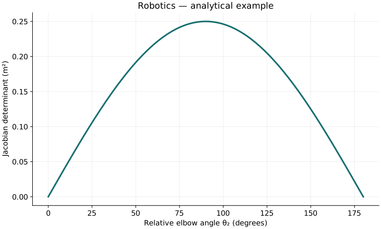
A straight or folded elbow loses one instantaneous position degree of freedom.
Interpretation. Near singularities, small endpoint commands can demand large joint motion.
↑ Return to definitions and contents3. Mobile motion and actuator dynamics
Definitions & inputs. r wheel radius, b track width, ωR,ωL wheel speeds; Jrot inertia; τ torque.
Average wheel speed translates; the difference rotates.
Net torque changes angular acceleration.
Mechanical power is torque times angular speed.
Interpretation. Traction, gearbox loss, saturation, and coupling affect real response.
↑ Return to definitions and contents4. Feedback and uncertainty
Definitions & inputs. e reference minus measurement, Kp proportional gain, R sensor variance, P prior estimate variance.
Proportional action maps tracking error into command.
A scalar Kalman update weights an independent measurement by relative uncertainty.
The posterior variance decreases under the stated independent Gaussian model.
Interpretation. Accurate static calibration does not replace dynamic control validation.
↑ Return to definitions and contentsGraphical worked example
Twenty worked examples
Open a problem to see its defined inputs, assumptions, equation, numerical substitution, result, and interpretation. Values are illustrative analytical exercises.
Example 01. One-link endpoint x
Definitions & inputs. l=0.5 m, θ=60°.
Choose the governing model and isolate the requested quantity.
Insert the stated inputs in consistent units or the explicitly defined normalized units.
Evaluate the expression; the result uses the units shown.
Interpretation. The y coordinate is positive and must be computed separately.
↑ Return to definitions and contentsExample 02. One-link endpoint y
Definitions & inputs. l=0.5 m, θ=60°.
Choose the governing model and isolate the requested quantity.
Insert the stated inputs in consistent units or the explicitly defined normalized units.
Evaluate the expression; the result uses the units shown.
Interpretation. Both coordinates refer to the same base frame.
↑ Return to definitions and contentsExample 03. Two-link endpoint x
Definitions & inputs. l1=l2=0.5 m, θ1=0°, θ2=90°.
Choose the governing model and isolate the requested quantity.
Insert the stated inputs in consistent units or the explicitly defined normalized units.
Evaluate the expression; the result uses the units shown.
Interpretation. The endpoint also has y=0.5 m.
↑ Return to definitions and contentsExample 04. Elbow inverse angle
Definitions & inputs. x=y=0.5 m, l1=l2=0.5 m; positive elbow branch.
Choose the governing model and isolate the requested quantity.
Insert the stated inputs in consistent units or the explicitly defined normalized units.
Evaluate the expression; the result uses the units shown.
Interpretation. The negative elbow branch is another possible configuration.
↑ Return to definitions and contentsExample 05. Reachability bound
Definitions & inputs. l1=0.4 m, l2=0.3 m.
Choose the governing model and isolate the requested quantity.
Insert the stated inputs in consistent units or the explicitly defined normalized units.
Evaluate the expression; the result uses the units shown.
Interpretation. The minimum reachable radius is |0.4−0.3|=0.1 m, before joint limits.
↑ Return to definitions and contentsExample 06. Single-link tangential speed
Definitions & inputs. l=0.5 m, angular rate=2 rad/s.
Choose the governing model and isolate the requested quantity.
Insert the stated inputs in consistent units or the explicitly defined normalized units.
Evaluate the expression; the result uses the units shown.
Interpretation. Direction is tangent to the circle, not always along x.
↑ Return to definitions and contentsExample 07. Static joint torque
Definitions & inputs. Perpendicular endpoint force F=10 N, arm l=0.4 m.
Choose the governing model and isolate the requested quantity.
Insert the stated inputs in consistent units or the explicitly defined normalized units.
Evaluate the expression; the result uses the units shown.
Interpretation. Nonperpendicular force requires the moment-arm sine factor.
↑ Return to definitions and contentsExample 08. Angular acceleration
Definitions & inputs. Net torque 2 N m, inertia 0.1 kg m².
Choose the governing model and isolate the requested quantity.
Insert the stated inputs in consistent units or the explicitly defined normalized units.
Evaluate the expression; the result uses the units shown.
Interpretation. Load torque has already been subtracted.
↑ Return to definitions and contentsExample 09. Motor mechanical power
Definitions & inputs. Torque 0.5 N m, speed 100 rad/s.
Choose the governing model and isolate the requested quantity.
Insert the stated inputs in consistent units or the explicitly defined normalized units.
Evaluate the expression; the result uses the units shown.
Interpretation. Electrical input is larger when efficiency is below one.
↑ Return to definitions and contentsExample 10. Gear output torque
Definitions & inputs. Input torque 0.2 N m, speed-reduction ratio 10, efficiency 0.9.
Choose the governing model and isolate the requested quantity.
Insert the stated inputs in consistent units or the explicitly defined normalized units.
Evaluate the expression; the result uses the units shown.
Interpretation. Output speed is one tenth of input under this ratio convention.
↑ Return to definitions and contentsExample 11. Encoder angular step
Definitions & inputs. 4096 resolved counts per revolution.
Choose the governing model and isolate the requested quantity.
Insert the stated inputs in consistent units or the explicitly defined normalized units.
Evaluate the expression; the result uses the units shown.
Interpretation. Resolved counts already include any quadrature multiplication.
↑ Return to definitions and contentsExample 12. Wheel travel
Definitions & inputs. Radius 0.1 m, rotation 3 revolutions.
Choose the governing model and isolate the requested quantity.
Insert the stated inputs in consistent units or the explicitly defined normalized units.
Evaluate the expression; the result uses the units shown.
Interpretation. Slip breaks the rolling-distance relation.
↑ Return to definitions and contentsExample 13. Differential-drive speed
Definitions & inputs. r=0.1 m; ωR=12, ωL=8 rad/s.
Choose the governing model and isolate the requested quantity.
Insert the stated inputs in consistent units or the explicitly defined normalized units.
Evaluate the expression; the result uses the units shown.
Interpretation. This is centre-point forward speed.
↑ Return to definitions and contentsExample 14. Differential-drive yaw rate
Definitions & inputs. Same wheels; track width b=0.5 m.
Choose the governing model and isolate the requested quantity.
Insert the stated inputs in consistent units or the explicitly defined normalized units.
Evaluate the expression; the result uses the units shown.
Interpretation. Sign is positive for the defined right-minus-left convention.
↑ Return to definitions and contentsExample 15. Stopping distance
Definitions & inputs. Initial speed 2 m/s; constant braking deceleration magnitude 1 m/s².
Choose the governing model and isolate the requested quantity.
Insert the stated inputs in consistent units or the explicitly defined normalized units.
Evaluate the expression; the result uses the units shown.
Interpretation. Reaction time adds distance before braking starts.
↑ Return to definitions and contentsExample 16. Triangular move duration
Definitions & inputs. Rest-to-rest distance 1 m, acceleration limit 2 m/s², no velocity cap reached.
Choose the governing model and isolate the requested quantity.
Insert the stated inputs in consistent units or the explicitly defined normalized units.
Evaluate the expression; the result uses the units shown.
Interpretation. Acceleration switches sign halfway through the motion.
↑ Return to definitions and contentsExample 17. Proportional control command
Definitions & inputs. Position error 0.05 rad, Kp=20 N m/rad.
Choose the governing model and isolate the requested quantity.
Insert the stated inputs in consistent units or the explicitly defined normalized units.
Evaluate the expression; the result uses the units shown.
Interpretation. This is a command before actuator limits.
↑ Return to definitions and contentsExample 18. Scalar estimator gain
Definitions & inputs. Prior variance P=4 mm², measurement variance R=1 mm².
Choose the governing model and isolate the requested quantity.
Insert the stated inputs in consistent units or the explicitly defined normalized units.
Evaluate the expression; the result uses the units shown.
Interpretation. The sensor receives most of the weight because its variance is smaller.
↑ Return to definitions and contentsExample 19. Posterior position estimate
Definitions & inputs. Prior 10 mm, measurement 12 mm, gain K=0.8.
Choose the governing model and isolate the requested quantity.
Insert the stated inputs in consistent units or the explicitly defined normalized units.
Evaluate the expression; the result uses the units shown.
Interpretation. The estimate lies between prior and measurement.
↑ Return to definitions and contentsExample 20. Jacobian singularity measure
Definitions & inputs. Planar 2R: l1=l2=0.5 m, θ2=0.
Choose the governing model and isolate the requested quantity.
Insert the stated inputs in consistent units or the explicitly defined normalized units.
Evaluate the expression; the result uses the units shown.
Interpretation. A straight elbow is position-singular; a pseudoinverse needs care.
↑ Return to definitions and contentsSymbols and units
Each derivation and problem defines its own symbols and inputs. Symbols may be reused with different meanings in other subjects. Keep units consistent, retain sufficient precision during calculation, and apply the stated validity limits.