PHYSICS / ENGINEERING / COMPUTING
Fluid mechanics models
Connect conservation laws to hydrostatics, pipe flow, boundary forces and compressibility with twenty worked examples.
Matter pathway: atom → solid → liquid → gas → plasma. Quantum mechanics and quantum field theory provide foundations across the pathway; they are not additional phases. This is a connected modeling route, not a universal heating curve. Actual phases depend on pressure, composition, and kinetics.
1. Mass and momentum
Definitions & inputs. ρ density, u velocity, p pressure, μ dynamic viscosity, g body acceleration.
Local mass conservation balances storage and flux.
For incompressible flow, pressure, viscous and body forces set acceleration.
Constant density reduces continuity and gives the uniform-section volume flux.
Interpretation. Compressible flow retains density variation and generally needs an energy equation.
↑ Return to definitions and contents2. Hydrostatics and energy
Definitions & inputs. z elevation, g gravity, V displaced volume, v speed.
Static momentum balance relates pressure to elevation.
Integrating hydrostatic traction gives buoyancy.
Dot inviscid momentum with the streamline displacement and integrate.
Interpretation. Pumps, viscous losses and heat/compressibility effects require a generalized energy balance.
↑ Return to definitions and contents3. Viscous pipe flow
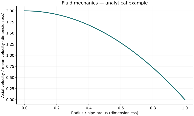
Definitions & inputs. R radius,L pipe length,Δp pressure drop,D=2R,vmean average velocity.
Axial momentum reduces to a radial differential equation.
Integrate using finite centreline gradient and zero wall velocity.
Integrate velocity over the cross section and express the result as a Darcy friction factor.
Interpretation. Do not use the laminar relation indiscriminately in transitional or turbulent flow.
↑ Return to definitions and contents4. Similarity and force
Definitions & inputs. Re Reynolds number, Cd drag coefficient, A frontal area, a sound speed, γ specific heat ratio.
Compare inertia with viscosity and flow speed with wave speed.
Define drag relative to dynamic pressure and reference area.
Linearize pressure-density response for an ideal gas under isentropic small disturbances.
Interpretation. Similarity parameters guide model selection; drag coefficients are not universal constants.
↑ Return to definitions and contentsGraphical worked example
Twenty worked examples
Open a problem to see its defined inputs, assumptions, equation, numerical substitution, result, and interpretation. Values are illustrative analytical exercises.
Example 01. Hydrostatic gauge pressure
Definitions & inputs. Water ρ=1000 kg/m³,depth 2 m,g=9.81 m/s².
Choose the governing model and isolate the requested quantity.
Insert the stated inputs in consistent units or the explicitly defined normalized units.
Evaluate the expression; the result uses the units shown.
Interpretation. Absolute pressure additionally includes surface pressure.
↑ Return to definitions and contentsExample 02. Buoyant force
Definitions & inputs. Displaced water volume .003 m³,ρ=1000 kg/m³.
Choose the governing model and isolate the requested quantity.
Insert the stated inputs in consistent units or the explicitly defined normalized units.
Evaluate the expression; the result uses the units shown.
Interpretation. Compare this upward force with weight and other loads.
↑ Return to definitions and contentsExample 03. Mass flow rate
Definitions & inputs. ρ=1000 kg/m³,Q=.002 m³/s.
Choose the governing model and isolate the requested quantity.
Insert the stated inputs in consistent units or the explicitly defined normalized units.
Evaluate the expression; the result uses the units shown.
Interpretation. Density must match the section where Q is specified.
↑ Return to definitions and contentsExample 04. Pipe velocity
Definitions & inputs. Q=.001 m³/s,D=.02 m.
Choose the governing model and isolate the requested quantity.
Insert the stated inputs in consistent units or the explicitly defined normalized units.
Evaluate the expression; the result uses the units shown.
Interpretation. This is area-averaged velocity.
↑ Return to definitions and contentsExample 05. Contraction velocity
Definitions & inputs. A1=.02 m²,v1=1 m/s,A2=.005 m².
Choose the governing model and isolate the requested quantity.
Insert the stated inputs in consistent units or the explicitly defined normalized units.
Evaluate the expression; the result uses the units shown.
Interpretation. Constant density and no branches are assumed.
↑ Return to definitions and contentsExample 06. Dynamic pressure
Definitions & inputs. Air ρ=1.2 kg/m³,v=20 m/s.
Choose the governing model and isolate the requested quantity.
Insert the stated inputs in consistent units or the explicitly defined normalized units.
Evaluate the expression; the result uses the units shown.
Interpretation. This is not the static pressure.
↑ Return to definitions and contentsExample 07. Ideal efflux speed
Definitions & inputs. Liquid head h=2 m,large tank,negligible losses.
Choose the governing model and isolate the requested quantity.
Insert the stated inputs in consistent units or the explicitly defined normalized units.
Evaluate the expression; the result uses the units shown.
Interpretation. A discharge coefficient is required for a real opening.
↑ Return to definitions and contentsExample 08. Horizontal Bernoulli pressure drop
Definitions & inputs. Water,v1=1 m/s,v2=3 m/s,no loss.
Choose the governing model and isolate the requested quantity.
Insert the stated inputs in consistent units or the explicitly defined normalized units.
Evaluate the expression; the result uses the units shown.
Interpretation. Static pressure falls where the flow speeds up.
↑ Return to definitions and contentsExample 09. Reynolds number
Definitions & inputs. ρ=1000 kg/m³,v=.1 m/s,D=.01 m,μ=.001 Pa s.
Choose the governing model and isolate the requested quantity.
Insert the stated inputs in consistent units or the explicitly defined normalized units.
Evaluate the expression; the result uses the units shown.
Interpretation. This is within the usual laminar circular-pipe regime for smooth disturbances.
↑ Return to definitions and contentsExample 10. Kinematic viscosity
Definitions & inputs. μ=.001 Pa s,ρ=1000 kg/m³.
Choose the governing model and isolate the requested quantity.
Insert the stated inputs in consistent units or the explicitly defined normalized units.
Evaluate the expression; the result uses the units shown.
Interpretation. Kinematic viscosity controls viscous momentum diffusion.
↑ Return to definitions and contentsExample 11. Laminar Darcy factor
Definitions & inputs. Re=1000.
Choose the governing model and isolate the requested quantity.
Insert the stated inputs in consistent units or the explicitly defined normalized units.
Evaluate the expression; the result uses the units shown.
Interpretation. The Fanning factor would be four times smaller.
↑ Return to definitions and contentsExample 12. Poiseuille flow
Definitions & inputs. R=.001 m,L=1 m,μ=.001 Pa s,Δp=100 Pa.
Choose the governing model and isolate the requested quantity.
Insert the stated inputs in consistent units or the explicitly defined normalized units.
Evaluate the expression; the result uses the units shown.
Interpretation. The implied Reynolds number is small, consistent with laminar flow.
↑ Return to definitions and contentsExample 13. Laminar peak velocity
Definitions & inputs. Mean velocity .2 m/s,fully developed circular pipe.
Choose the governing model and isolate the requested quantity.
Insert the stated inputs in consistent units or the explicitly defined normalized units.
Evaluate the expression; the result uses the units shown.
Interpretation. The profile is parabolic under these assumptions.
↑ Return to definitions and contentsExample 14. Pipe wall shear
Definitions & inputs. Δp=100 Pa,D=.01 m,L=2 m.
Choose the governing model and isolate the requested quantity.
Insert the stated inputs in consistent units or the explicitly defined normalized units.
Evaluate the expression; the result uses the units shown.
Interpretation. This follows an axial force balance in fully developed flow.
↑ Return to definitions and contentsExample 15. Darcy head loss
Definitions & inputs. fD=.02,L=10 m,D=.1 m,v=2 m/s.
Choose the governing model and isolate the requested quantity.
Insert the stated inputs in consistent units or the explicitly defined normalized units.
Evaluate the expression; the result uses the units shown.
Interpretation. The supplied friction factor must be appropriate for roughness and Reynolds number.
↑ Return to definitions and contentsExample 16. Pump shaft power
Definitions & inputs. Δp=100 kPa,Q=.01 m³/s,efficiency .7.
Choose the governing model and isolate the requested quantity.
Insert the stated inputs in consistent units or the explicitly defined normalized units.
Evaluate the expression; the result uses the units shown.
Interpretation. Hydraulic power is 1000 W; shaft power includes loss.
↑ Return to definitions and contentsExample 17. Drag force
Definitions & inputs. ρ=1.2 kg/m³,v=20 m/s,A=.5 m²,Cd=1.
Choose the governing model and isolate the requested quantity.
Insert the stated inputs in consistent units or the explicitly defined normalized units.
Evaluate the expression; the result uses the units shown.
Interpretation. Cd is an input specific to the body and flow.
↑ Return to definitions and contentsExample 18. Mach number
Definitions & inputs. v=170 m/s,a=340 m/s.
Choose the governing model and isolate the requested quantity.
Insert the stated inputs in consistent units or the explicitly defined normalized units.
Evaluate the expression; the result uses the units shown.
Interpretation. Compressibility may be significant at this Mach number.
↑ Return to definitions and contentsExample 19. Ideal-gas sound speed
Definitions & inputs. γ=1.4,Rs=287 J/(kg K),T=300 K.
Choose the governing model and isolate the requested quantity.
Insert the stated inputs in consistent units or the explicitly defined normalized units.
Evaluate the expression; the result uses the units shown.
Interpretation. Thermodynamic composition and temperature set γ and Rs.
↑ Return to definitions and contentsExample 20. Capillary rise
Definitions & inputs. Surface tension .072 N/m,contact angle 0°,radius .001 m,ρ=1000 kg/m³.
Choose the governing model and isolate the requested quantity.
Insert the stated inputs in consistent units or the explicitly defined normalized units.
Evaluate the expression; the result uses the units shown.
Interpretation. The tube is narrow enough for capillarity and the meniscus contact angle is prescribed.
↑ Return to definitions and contentsSymbols and units
Each derivation and problem defines its own symbols and inputs. Symbols may be reused with different meanings in other subjects. Keep units consistent, retain sufficient precision during calculation, and apply the stated validity limits.