PHYSICS / ENGINEERING / COMPUTING
Ship design: buoyancy, stability, resistance and power
Connect hull geometry and displacement to initial stability, hydrodynamic resistance, propulsion and structural response.
Matter pathway: atom → solid → liquid → gas → plasma. Quantum mechanics and quantum field theory provide foundations across the pathway; they are not additional phases. This is a connected modeling route, not a universal heating curve. Actual phases depend on pressure, composition, and kinetics.
1. Hydrostatics and displacement
Definitions & inputs. ρ water density,g gravity,∇ displaced volume,m vessel mass,L length,B beam,T draft,CB block coefficient.
Integrate hydrostatic pressure to obtain Archimedes’ buoyancy.
The block coefficient describes volume relative to the enclosing box.
A small added mass sinks a vessel according to waterplane area.
Interpretation. Waterplane area changes with draft, so large loading changes require the actual hydrostatic curves.
↑ Return to definitions and contents2. Initial transverse stability
Definitions & inputs. KB center of buoyancy height,KG center of gravity height,Iwp transverse waterplane second moment,GM metacentric height,φ heel.
Small heel shifts the center of buoyancy and defines the metacenter.
The horizontal buoyancy-weight lever gives righting moment.
Liquid free surfaces reduce initial stability.
Interpretation. Positive GM alone does not establish large-angle stability, downflooding margin or damage survivability.
↑ Return to definitions and contents3. Resistance and propulsion
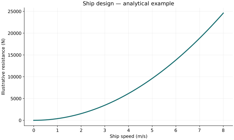
Definitions & inputs. R total resistance,V speed,ρ density,S wetted area,CT coefficient,ηD propulsive efficiency.
A nondimensional resistance coefficient scales the force.
Tow power becomes delivered shaft power after propulsive losses.
Viscous and gravity-wave similarity cannot generally both match in a small-scale water model.
Interpretation. Propeller open-water maps, wake, thrust deduction and cavitation must be evaluated rather than replacing every loss by one constant efficiency.
↑ Return to definitions and contents4. Structure and seakeeping
Definitions & inputs. M hull bending moment,I section second moment,y distance from neutral axis,k wave number,ω wave frequency,h water depth.
Global hull-girder bending produces longitudinal stress.
Linear gravity-wave dispersion connects wavelength and frequency.
Encounter frequency depends on vessel motion relative to wave propagation directionβ.
Interpretation. Slamming, whipping, corrosion, fatigue and local buckling need additional load cases and models.
↑ Return to definitions and contentsGraphical worked example
Twenty worked examples
Open a problem to see its defined inputs, assumptions, equation, numerical substitution, result, and interpretation. Values are illustrative analytical exercises.
Example 01. Displaced volume
Definitions & inputs. L20m,B5m,T2m,CB.6.
Choose the governing model and isolate the requested quantity.
Insert the stated inputs in consistent units or the explicitly defined normalized units.
Evaluate the expression; the result uses the units shown.
Interpretation. Simple block-coefficient model.
↑ Return to definitions and contentsExample 02. Displacement mass
Definitions & inputs. Seawater1025kg/m³,volume120m³.
Choose the governing model and isolate the requested quantity.
Insert the stated inputs in consistent units or the explicitly defined normalized units.
Evaluate the expression; the result uses the units shown.
Interpretation. Static flotation.
↑ Return to definitions and contentsExample 03. Buoyancy force
Definitions & inputs. Same volume,g9.81.
Choose the governing model and isolate the requested quantity.
Insert the stated inputs in consistent units or the explicitly defined normalized units.
Evaluate the expression; the result uses the units shown.
Interpretation. Equal to weight at equilibrium.
↑ Return to definitions and contentsExample 04. Freshwater volume
Definitions & inputs. Mass123000kg,ρ1000.
Choose the governing model and isolate the requested quantity.
Insert the stated inputs in consistent units or the explicitly defined normalized units.
Evaluate the expression; the result uses the units shown.
Interpretation. More volume must be displaced than in seawater.
↑ Return to definitions and contentsExample 05. Draft increment
Definitions & inputs. Added mass1000kg,Awp80m²,ρ1025.
Choose the governing model and isolate the requested quantity.
Insert the stated inputs in consistent units or the explicitly defined normalized units.
Evaluate the expression; the result uses the units shown.
Interpretation. Small increment only.
↑ Return to definitions and contentsExample 06. Rectangular waterplane inertia
Definitions & inputs. L20m,B5m.
Choose the governing model and isolate the requested quantity.
Insert the stated inputs in consistent units or the explicitly defined normalized units.
Evaluate the expression; the result uses the units shown.
Interpretation. Roll about longitudinal axis.
↑ Return to definitions and contentsExample 07. Metacentric radius
Definitions & inputs. Iwp208.333m⁴,volume120m³.
Choose the governing model and isolate the requested quantity.
Insert the stated inputs in consistent units or the explicitly defined normalized units.
Evaluate the expression; the result uses the units shown.
Interpretation. Idealized waterplane.
↑ Return to definitions and contentsExample 08. Metacentric height
Definitions & inputs. KB1m,BM1.7m,KG2m.
Choose the governing model and isolate the requested quantity.
Insert the stated inputs in consistent units or the explicitly defined normalized units.
Evaluate the expression; the result uses the units shown.
Interpretation. Positive initial stability.
↑ Return to definitions and contentsExample 09. Small-angle righting arm
Definitions & inputs. GM.7m,heel5°.
Choose the governing model and isolate the requested quantity.
Insert the stated inputs in consistent units or the explicitly defined normalized units.
Evaluate the expression; the result uses the units shown.
Interpretation. Small-angle approximation.
↑ Return to definitions and contentsExample 10. Righting moment
Definitions & inputs. m123000kg,GM.7m,heel5°.
Choose the governing model and isolate the requested quantity.
Insert the stated inputs in consistent units or the explicitly defined normalized units.
Evaluate the expression; the result uses the units shown.
Interpretation. Intact illustrative loading.
↑ Return to definitions and contentsExample 11. Free-surface correction
Definitions & inputs. ρtank1000,I10m⁴,displaced mass123000kg.
Choose the governing model and isolate the requested quantity.
Insert the stated inputs in consistent units or the explicitly defined normalized units.
Evaluate the expression; the result uses the units shown.
Interpretation. Subtract from uncorrected GM.
↑ Return to definitions and contentsExample 12. Froude number
Definitions & inputs. V5m/s,L20m.
Choose the governing model and isolate the requested quantity.
Insert the stated inputs in consistent units or the explicitly defined normalized units.
Evaluate the expression; the result uses the units shown.
Interpretation. Gravity-wave similarity.
↑ Return to definitions and contentsExample 13. Reynolds number
Definitions & inputs. V5m/s,L20m,ν10⁻⁶m²/s.
Choose the governing model and isolate the requested quantity.
Insert the stated inputs in consistent units or the explicitly defined normalized units.
Evaluate the expression; the result uses the units shown.
Interpretation. Viscous similarity.
↑ Return to definitions and contentsExample 14. Resistance
Definitions & inputs. ρ1025,V5,S150m²,CT.005.
Choose the governing model and isolate the requested quantity.
Insert the stated inputs in consistent units or the explicitly defined normalized units.
Evaluate the expression; the result uses the units shown.
Interpretation. Assumed fitted CT.
↑ Return to definitions and contentsExample 15. Effective power
Definitions & inputs. R10000N,V5m/s.
Choose the governing model and isolate the requested quantity.
Insert the stated inputs in consistent units or the explicitly defined normalized units.
Evaluate the expression; the result uses the units shown.
Interpretation. Tow power.
↑ Return to definitions and contentsExample 16. Delivered shaft power
Definitions & inputs. PE50kW,ηD.6.
Choose the governing model and isolate the requested quantity.
Insert the stated inputs in consistent units or the explicitly defined normalized units.
Evaluate the expression; the result uses the units shown.
Interpretation. Simplified efficiency budget.
↑ Return to definitions and contentsExample 17. Propeller advance ratio
Definitions & inputs. V advance5m/s,n5rev/s,D2m.
Choose the governing model and isolate the requested quantity.
Insert the stated inputs in consistent units or the explicitly defined normalized units.
Evaluate the expression; the result uses the units shown.
Interpretation. Use advance velocity not blindly ship speed.
↑ Return to definitions and contentsExample 18. Hull beam stress
Definitions & inputs. M10⁶Nm,y1m,I.1m⁴.
Choose the governing model and isolate the requested quantity.
Insert the stated inputs in consistent units or the explicitly defined normalized units.
Evaluate the expression; the result uses the units shown.
Interpretation. Linear global bending.
↑ Return to definitions and contentsExample 19. Deep-water wavelength
Definitions & inputs. Period8s.
Choose the governing model and isolate the requested quantity.
Insert the stated inputs in consistent units or the explicitly defined normalized units.
Evaluate the expression; the result uses the units shown.
Interpretation. Deep-water linear wave approximation.
↑ Return to definitions and contentsExample 20. Added-load margin
Definitions & inputs. Mass limit150t,current123t.
Choose the governing model and isolate the requested quantity.
Insert the stated inputs in consistent units or the explicitly defined normalized units.
Evaluate the expression; the result uses the units shown.
Interpretation. Mass budget only; not stability approval.
↑ Return to definitions and contentsSymbols and units
Each derivation and problem defines its own symbols and inputs. Symbols may be reused with different meanings in other subjects. Keep units consistent, retain sufficient precision during calculation, and apply the stated validity limits.