PHYSICS / ENGINEERING / COMPUTING
Materials science models
Link atomic structure and microstructure to diffusion, mixtures, thermal response, fracture and fatigue through twenty worked examples.
Matter pathway: atom → solid → liquid → gas → plasma. Quantum mechanics and quantum field theory provide foundations across the pathway; they are not additional phases. This is a connected modeling route, not a universal heating curve. Actual phases depend on pressure, composition, and kinetics.
Material families and model-selection map
Choose the family, processing route, scale and service environment before choosing a constitutive equation. The examples below identify familiar applications, not grade-specific design allowables.
- Metals and alloys
- FCC/BCC/HCP structure, dislocations, solid solutions, precipitation, recovery and recrystallization. Examples: aluminum airframes, steel vehicle bodies, nickel-superalloy turbine components. Resolve texture and temperature when isotropic elasticity or a single yield stress is inadequate.
- Ceramics and glasses
- Ionic/covalent bonding, brittle fracture statistics, sintering and slow crack growth. Examples: alumina electrical insulators, zirconia dental components, silica optical fibers. Distinguish crystalline grains from amorphous glass and surface-flaw-controlled failure.
- Polymers and elastomers
- Chain structure, crystallinity, glass transition, viscoelasticity, rubber elasticity and aging. Examples: polyethylene packaging, epoxy adhesives, silicone seals. Time, temperature, humidity and loading rate affect response.
- Composites and cellular materials
- Fibers, particles, laminates, interfaces, foam cells, anisotropy and damage. Examples: carbon-fiber aircraft panels, glass-fiber wind blades, sandwich cores. Homogenized mixture bounds do not predict delamination or every directional property.
- Semiconductors and functional materials
- Band structure, charge carriers, dielectric polarization, ferroelectricity, magnetic domains and piezoelectric coupling. Examples: silicon processors, SiC power electronics, PZT actuators, ferrite cores. Couple electrical, thermal and mechanical fields where necessary.
- Energy and environmental materials
- Ion diffusion, electrochemical potentials, phase separation, corrosion, passivation and swelling. Examples: lithium-ion electrodes, fuel-cell membranes and corrosion-resistant piping. Transport and reaction models must share consistent species and charge balances.
- Interfaces, nanoscale and biomaterials
- Surface energy, adhesion, size effects and interaction with biological environments. Examples: thin-film coatings, implant alloys and hydrogel devices. Bulk continuum coefficients can fail at small scales.
Characterization connects the model to evidence
X-ray diffraction tests structure and phases; microscopy and EBSD reveal grains and texture; calorimetry identifies transitions; tensile, creep and dynamic-mechanical tests calibrate mechanical laws; spectroscopy and transport measurements test electronic models. Report specimen orientation, processing history, uncertainty and test temperature alongside fitted coefficients.
Plastic and viscoelastic deformation · Continuum mechanics · Solid-state physics · Reaction kinetics
1. Atomic structure and density
Definitions & inputs. n atoms/unit cell,M molar mass,NA Avogadro constant,a cubic lattice parameter.
Convert a count of atoms into cell mass.
Divide cell mass by cell volume.
Cubic reciprocal-lattice geometry gives plane spacing.
Interpretation. Vacancies, alloy composition and thermal expansion alter density and diffraction positions.
↑ Return to definitions and contents2. Diffusion and kinetics
Definitions & inputs. J molar flux,D diffusivity,c concentration,Dt time-diffusion product.
Concentration gradients drive down-gradient transport.
Combine the flux law with conservation.
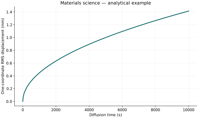
Random-walk spreading in one coordinate and activated hopping set distance and temperature dependence.
Interpretation. Short-circuit paths, stress and composition dependence can require a more detailed transport model.
↑ Return to definitions and contents3. Mixtures and microstructure
Definitions & inputs. Vf constituent volume fraction,E1,E2 elastic moduli,d grain size,kHP Hall–Petch coefficient.
Shared strain adds constituent stresses, producing the Voigt estimate.
Shared stress adds constituent strains, producing the Reuss estimate.
An empirical grain-size relation describes strengthening in an appropriate regime.
Interpretation. These ideal bounds and correlations do not replace a measured anisotropic composite response.
↑ Return to definitions and contents4. Failure and time dependence
Definitions & inputs. KI crack intensity,Y geometry factor,a crack length,KIC toughness,σa fatigue stress amplitude.
The near-tip elastic singularity scales with remote stress and crack size.
Set the intensity equal to the fracture toughness and solve for crack size.
A Basquin fit relates elastic fatigue amplitude to reversals to failure.
Interpretation. Toughness, crack geometry, plasticity, environment and fatigue scatter must be checked independently.
↑ Return to definitions and contents5. Point defects and site occupancy
Definitions & inputs. cv vacancy fraction,ΔGf formation free energy,kB Boltzmann constant.
Separate energetic and entropic contributions to forming a defect.
Minimize the dilute defect free energy including configurational entropy.
Substitute kB=8.617333262×10⁻⁵eV/K for a checkable toy value.
Interpretation. Vacancies enable diffusion; dislocations accommodate slip; grain boundaries introduce distinct mobility and segregation pathways.
↑ Return to definitions and contents6. Phase equilibrium and tie lines
Definitions & inputs. G Gibbs energy,μi chemical potential,C composition on a single consistent mass or mole basis,f phase fraction.
Transfer of a species cannot lower total Gibbs energy at coexistence.
Conserve composition across two phases.
Derive the lever rule and apply the existing worked example.
Interpretation. Phase fraction is not generally volume fraction unless densities and composition conventions support that conversion. Equilibrium phase diagrams do not alone predict transformation speed.
↑ Return to definitions and contents7. Nucleation and transformation
Definitions & inputs. γ interface energy,Δgv negative bulk free-energy change per volume,r nucleus radius,X transformed fraction.
Competing surface cost and bulk benefit create a barrier.
Differentiate with respect to r and substitute the stationary radius.
A numerical critical size and an independent Avrami transformation law illustrate the difference between nucleation and bulk kinetics.
Interpretation. Heterogeneous sites reduce barriers; martensitic, diffusion-controlled and glass transitions require different models. An atomic-scale nucleus challenges the continuum approximation.
↑ Return to definitions and contents8. Dislocations and slip systems
Definitions & inputs. τRSS resolved shear stress,σ uniaxial stress,φ angle to slip-plane normal,λ angle to slip direction,ρd dislocation line length per volume,b Burgers-vector magnitude,v glide speed.
Project traction onto the slip plane and slip direction.
Swept slip area per volume gives Orowan’s plastic shear rate.
Check that the line density, Burgers vector and velocity produce inverse-time units.
Interpretation. Work hardening, precipitates, solid-solution strengthening and grain boundaries impede different parts of this motion; one empirical strength law cannot identify all mechanisms.
↑ Return to definitions and contents9. Creep and high-temperature deformation
Definitions & inputs. εdot steady creep rate,A prefactor,σstress,n stress exponent,Q activation energy,R gas constant.
A Norton–Arrhenius law combines stress dependence and thermal activation.
Linearize to identify slopes only while the deformation mechanism remains unchanged.
Doubling stress can sharply increase the creep rate in this illustrative regime.
Interpretation. Diffusional creep, dislocation climb and grain-boundary sliding have different exponents and grain-size sensitivity. Creep rupture life is not obtained from a steady rate alone.
↑ Return to definitions and contents10. Electronic and thermal transport
Definitions & inputs. n electron density,p hole density,μe andμh mobilities,σel electrical conductivity,k thermal conductivity.
Sum carrier current responses to an electric field.
Fourier transport and the metallic electronic Lorenz relation connect different response coefficients.
Use q=1.602176634×10⁻¹⁹C and neglect holes for this example.
Interpretation. Band structure, doping, defects and phonon scattering set the coefficients. Si logic, SiC power devices and thermoelectric materials optimize different combinations.
↑ Return to definitions and contents11. Polymers and relaxation spectra
Definitions & inputs. E(t) relaxation modulus,E∞ long-time modulus,Ek modal stiffness,τk relaxation time.
A generalized Maxwell model resolves multiple relaxation processes.
Superpose responses to increments of strain history.
A one-mode example separates instantaneous and relaxed stiffness.
Interpretation. Thermoplastics, thermosets and elastomers differ in chain mobility and crosslinking; a glass-transition temperature depends on the measurement time scale.
↑ Return to definitions and contents12. Processing, porosity and material selection
Definitions & inputs. P porosity fraction,ρs fully dense density,E/ρ specific stiffness,σallow allowable stress under specified conditions.
Neglect pore-gas mass in a porous solid.
Combine density with component geometry to compare structural function rather than raw modulus alone.
For fixed axial stiffness and length, minimize ρ/E under the stated geometry model.
Interpretation. Additive manufacture, casting, forging, heat treatment, sintering, layup and machining change defects, texture, residual stress and tolerances. A different load mode leads to a different material index.
↑ Return to definitions and contentsGraphical worked example
Twenty worked examples
Open a problem to see its defined inputs, assumptions, equation, numerical substitution, result, and interpretation. Values are illustrative analytical exercises.
Example 01. Cubic crystal density
Definitions & inputs. FCC n=4,M=.063546 kg/mol,a=.3615 nm,NA=6.02214076×10²³/mol.
Choose the governing model and isolate the requested quantity.
Insert the stated inputs in consistent units or the explicitly defined normalized units.
Evaluate the expression; the result uses the units shown.
Interpretation. Ideal site occupancy and the stated lattice parameter are assumed.
↑ Return to definitions and contentsExample 02. Cubic (110) plane spacing
Definitions & inputs. a=.4 nm.
Choose the governing model and isolate the requested quantity.
Insert the stated inputs in consistent units or the explicitly defined normalized units.
Evaluate the expression; the result uses the units shown.
Interpretation. This is a cubic-lattice spacing formula.
↑ Return to definitions and contentsExample 03. First-order Bragg angle
Definitions & inputs. λ=.154 nm,d=.2 nm.
Choose the governing model and isolate the requested quantity.
Insert the stated inputs in consistent units or the explicitly defined normalized units.
Evaluate the expression; the result uses the units shown.
Interpretation. A diffraction instrument often reports 2θ rather than θ.
↑ Return to definitions and contentsExample 04. Vacancy equilibrium fraction
Definitions & inputs. Formation energy 1 eV,T=1000 K,kB=8.617333262×10⁻⁵ eV/K,prefactor one.
Choose the governing model and isolate the requested quantity.
Insert the stated inputs in consistent units or the explicitly defined normalized units.
Evaluate the expression; the result uses the units shown.
Interpretation. Formation entropy is neglected in this illustrative prefactor.
↑ Return to definitions and contentsExample 05. Fickian flux
Definitions & inputs. D=10⁻¹⁰ m²/s,dc/dx=1000 mol/m⁴.
Choose the governing model and isolate the requested quantity.
Insert the stated inputs in consistent units or the explicitly defined normalized units.
Evaluate the expression; the result uses the units shown.
Interpretation. The negative sign points toward lower concentration.
↑ Return to definitions and contentsExample 06. One-dimensional diffusion length
Definitions & inputs. D=10⁻¹⁰ m²/s,t=1000 s.
Choose the governing model and isolate the requested quantity.
Insert the stated inputs in consistent units or the explicitly defined normalized units.
Evaluate the expression; the result uses the units shown.
Interpretation. A three-dimensional radial RMS distance would use 6Dt.
↑ Return to definitions and contentsExample 07. Diffusion time estimate
Definitions & inputs. Desired one-dimensional RMS length 1 mm,D=10⁻¹⁰ m²/s.
Choose the governing model and isolate the requested quantity.
Insert the stated inputs in consistent units or the explicitly defined normalized units.
Evaluate the expression; the result uses the units shown.
Interpretation. This random-walk scale is not a complete finite-body concentration solution.
↑ Return to definitions and contentsExample 08. Activated diffusivity
Definitions & inputs. D0=10⁻⁵ m²/s,Q=100 kJ/mol,T=1000 K,R=8.314462618.
Choose the governing model and isolate the requested quantity.
Insert the stated inputs in consistent units or the explicitly defined normalized units.
Evaluate the expression; the result uses the units shown.
Interpretation. Mechanism and prefactor are assumed fixed over this temperature range.
↑ Return to definitions and contentsExample 09. Voigt composite modulus
Definitions & inputs. V1=.6,E1=200 GPa,E2=3 GPa.
Choose the governing model and isolate the requested quantity.
Insert the stated inputs in consistent units or the explicitly defined normalized units.
Evaluate the expression; the result uses the units shown.
Interpretation. Iso-strain loading is an ideal upper estimate under the stated scalar mixture model.
↑ Return to definitions and contentsExample 10. Reuss composite modulus
Definitions & inputs. Same V1=.6,E1=200,E2=3 GPa.
Choose the governing model and isolate the requested quantity.
Insert the stated inputs in consistent units or the explicitly defined normalized units.
Evaluate the expression; the result uses the units shown.
Interpretation. Iso-stress response gives a contrasting lower ideal estimate.
↑ Return to definitions and contentsExample 11. Mixture density
Definitions & inputs. V1=.6,ρ1=1800 kg/m³,ρ2=1200 kg/m³,no voids.
Choose the governing model and isolate the requested quantity.
Insert the stated inputs in consistent units or the explicitly defined normalized units.
Evaluate the expression; the result uses the units shown.
Interpretation. Fractions are by volume, not mass.
↑ Return to definitions and contentsExample 12. Hall–Petch strength
Definitions & inputs. σ0=50 MPa,kHP=.5 MPa√m,d=25 μm.
Choose the governing model and isolate the requested quantity.
Insert the stated inputs in consistent units or the explicitly defined normalized units.
Evaluate the expression; the result uses the units shown.
Interpretation. Extrapolation to extreme nanoscale grains is not justified by this example.
↑ Return to definitions and contentsExample 13. Lever-rule phase fraction
Definitions & inputs. Overall composition C0=40%,phase α Cα=20%,phase β Cβ=80%; same composition basis.
Choose the governing model and isolate the requested quantity.
Insert the stated inputs in consistent units or the explicitly defined normalized units.
Evaluate the expression; the result uses the units shown.
Interpretation. The tie line and phase compositions must correspond to equilibrium at the stated temperature.
↑ Return to definitions and contentsExample 14. Thermal free strain
Definitions & inputs. α=20×10⁻⁶/K,ΔT=100 K.
Choose the governing model and isolate the requested quantity.
Insert the stated inputs in consistent units or the explicitly defined normalized units.
Evaluate the expression; the result uses the units shown.
Interpretation. Restraint converts part of the free strain into mechanical stress.
↑ Return to definitions and contentsExample 15. Specific stiffness
Definitions & inputs. E=70 GPa,ρ=2700 kg/m³.
Choose the governing model and isolate the requested quantity.
Insert the stated inputs in consistent units or the explicitly defined normalized units.
Evaluate the expression; the result uses the units shown.
Interpretation. Component performance also depends on geometry and load mode.
↑ Return to definitions and contentsExample 16. Crack intensity
Definitions & inputs. Y=1,σ=100 MPa,a=.001 m.
Choose the governing model and isolate the requested quantity.
Insert the stated inputs in consistent units or the explicitly defined normalized units.
Evaluate the expression; the result uses the units shown.
Interpretation. Crack-length convention is part of the selected geometry factor.
↑ Return to definitions and contentsExample 17. Critical crack length
Definitions & inputs. KIC=30 MPa√m,Y=1,σ=100 MPa.
Choose the governing model and isolate the requested quantity.
Insert the stated inputs in consistent units or the explicitly defined normalized units.
Evaluate the expression; the result uses the units shown.
Interpretation. Small-scale yielding and the relevant toughness state are required.
↑ Return to definitions and contentsExample 18. Basquin fatigue amplitude
Definitions & inputs. σf′=1000 MPa,b=−.1,Nf=10⁶ cycles.
Choose the governing model and isolate the requested quantity.
Insert the stated inputs in consistent units or the explicitly defined normalized units.
Evaluate the expression; the result uses the units shown.
Interpretation. The law uses reversals 2Nf and ignores mean-stress correction here.
↑ Return to definitions and contentsExample 19. Linear creep extension
Definitions & inputs. Constant steady creep rate 10⁻⁸/s,t=10⁶ s,L=1 m.
Choose the governing model and isolate the requested quantity.
Insert the stated inputs in consistent units or the explicitly defined normalized units.
Evaluate the expression; the result uses the units shown.
Interpretation. Primary and tertiary creep are excluded.
↑ Return to definitions and contentsExample 20. Avrami transformed fraction
Definitions & inputs. X=1−exp(−ktⁿ),n=2,k=.01 s⁻²,t=10 s.
Choose the governing model and isolate the requested quantity.
Insert the stated inputs in consistent units or the explicitly defined normalized units.
Evaluate the expression; the result uses the units shown.
Interpretation. The fitted nucleation/growth model is limited to its calibrated transformation regime.
↑ Return to definitions and contentsSymbols and units
Each derivation and problem defines its own symbols and inputs. Symbols may be reused with different meanings in other subjects. Keep units consistent, retain sufficient precision during calculation, and apply the stated validity limits.