PHYSICS / ENGINEERING / COMPUTING
Internal combustion engine design
Derive ideal cycles, displacement, indicated and brake performance, mixture budgets and cooling loads.
Matter pathway: atom → solid → liquid → gas → plasma. Quantum mechanics and quantum field theory provide foundations across the pathway; they are not additional phases. This is a connected modeling route, not a universal heating curve. Actual phases depend on pressure, composition, and kinetics.
1. Geometry and four-stroke timing
Definitions & inputs. B bore,S stroke,nc cylinders,Vd swept volume,Vc clearance volume,N rev/s.
Swept and clearance volumes set compression ratio.
Intake, compression, expansion and exhaust occupy two crank revolutions.
Mean piston speed counts two strokes per revolution.
Interpretation. Piston acceleration, rod ratio, valve timing and breathing need more detailed kinematics and gas dynamics.
↑ Return to definitions and contents2. Otto cycle efficiency
Definitions & inputs. r compression ratio,γ heat capacity ratio,Qin andQout cycle heat.
Isentropic relations connect temperature to volume ratio.
Use the first law and constant cv heat transfers.
Eliminate temperatures using the matched isentropic ratios.
Interpretation. This efficiency is not a real brake efficiency or a recommendation to increase compression without knock analysis.
↑ Return to definitions and contents3. Diesel cycle and performance metrics
Definitions & inputs. rc cutoff ratio,Vd total displacement,imep andbmep indicated/brake mean effective pressures,τ shaft torque.
Substitute constant-pressure heat addition into the ideal cycle heat ratio.
Brake power equals torque speed or four-stroke brake work times cycles per second.
Separate indicated power from mechanical and pumping/friction accounting under a consistent convention.
Interpretation. A high mean effective pressure does not guarantee thermal efficiency or durability.
↑ Return to definitions and contents4. Fuel, mixture and thermal balance
Definitions & inputs. fuel mass flow rate fuel mass rate,LHV lower heating value,AFR air fuel ratio,λ excess air ratio.
Define brake thermal efficiency and brake-specific fuel consumption with consistent units.
Compare mixture with the fuel-specific stoichiometric ratio.
Account for all outgoing energy rather than equating ideal cycle efficiency with measured output.
Interpretation. Spark timing, injection, turbulence, heat transfer, catalyst temperature and control connect this subject to chemical kinetics, fluids and embedded systems.
↑ Return to definitions and contentsGraphical worked example
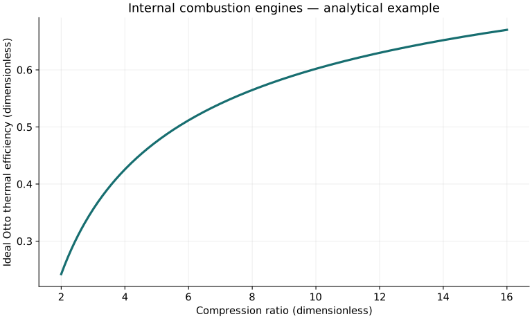
Twenty worked examples
Open a problem to see its defined inputs, assumptions, equation, numerical substitution, result, and interpretation. Values are illustrative analytical exercises.
Example 01. Single-cylinder displacement
Definitions & inputs. B.08m,S.09m.
Choose the governing model and isolate the requested quantity.
Insert the stated inputs in consistent units or the explicitly defined normalized units.
Evaluate the expression; the result uses the units shown.
Interpretation. Cubic meters converted to cubic centimeters.
↑ Return to definitions and contentsExample 02. Four-cylinder displacement
Definitions & inputs. Same bore stroke,nc4.
Choose the governing model and isolate the requested quantity.
Insert the stated inputs in consistent units or the explicitly defined normalized units.
Evaluate the expression; the result uses the units shown.
Interpretation. Liters conversion.
↑ Return to definitions and contentsExample 03. Compression ratio
Definitions & inputs. Vs500cm³,Vc50cm³.
Choose the governing model and isolate the requested quantity.
Insert the stated inputs in consistent units or the explicitly defined normalized units.
Evaluate the expression; the result uses the units shown.
Interpretation. Per-cylinder volumes.
↑ Return to definitions and contentsExample 04. Clearance volume
Definitions & inputs. Vs500cm³,r10.
Choose the governing model and isolate the requested quantity.
Insert the stated inputs in consistent units or the explicitly defined normalized units.
Evaluate the expression; the result uses the units shown.
Interpretation. Positive clearance.
↑ Return to definitions and contentsExample 05. Revolutions per second
Definitions & inputs. n3000rpm.
Choose the governing model and isolate the requested quantity.
Insert the stated inputs in consistent units or the explicitly defined normalized units.
Evaluate the expression; the result uses the units shown.
Interpretation. Crank speed.
↑ Return to definitions and contentsExample 06. Four-stroke cycle rate
Definitions & inputs. N50rev/s.
Choose the governing model and isolate the requested quantity.
Insert the stated inputs in consistent units or the explicitly defined normalized units.
Evaluate the expression; the result uses the units shown.
Interpretation. Per-cylinder firing cycle frequency.
↑ Return to definitions and contentsExample 07. Mean piston speed
Definitions & inputs. S.09m,N50/s.
Choose the governing model and isolate the requested quantity.
Insert the stated inputs in consistent units or the explicitly defined normalized units.
Evaluate the expression; the result uses the units shown.
Interpretation. Mean absolute piston speed.
↑ Return to definitions and contentsExample 08. Ideal Otto efficiency
Definitions & inputs. r10,γ1.4.
Choose the governing model and isolate the requested quantity.
Insert the stated inputs in consistent units or the explicitly defined normalized units.
Evaluate the expression; the result uses the units shown.
Interpretation. Air-standard upper benchmark under these constraints.
↑ Return to definitions and contentsExample 09. Compressed temperature
Definitions & inputs. T1300K,r10,γ1.4.
Choose the governing model and isolate the requested quantity.
Insert the stated inputs in consistent units or the explicitly defined normalized units.
Evaluate the expression; the result uses the units shown.
Interpretation. Constant gamma approximation.
↑ Return to definitions and contentsExample 10. Compressed pressure
Definitions & inputs. p1100kPa,r10,γ1.4.
Choose the governing model and isolate the requested quantity.
Insert the stated inputs in consistent units or the explicitly defined normalized units.
Evaluate the expression; the result uses the units shown.
Interpretation. Ideal adiabatic compression.
↑ Return to definitions and contentsExample 11. Ideal Diesel efficiency
Definitions & inputs. r18,rc2,γ1.4.
Choose the governing model and isolate the requested quantity.
Insert the stated inputs in consistent units or the explicitly defined normalized units.
Evaluate the expression; the result uses the units shown.
Interpretation. Constant-pressure heat addition.
↑ Return to definitions and contentsExample 12. Brake power
Definitions & inputs. Torque100Nm,speed3000rpm.
Choose the governing model and isolate the requested quantity.
Insert the stated inputs in consistent units or the explicitly defined normalized units.
Evaluate the expression; the result uses the units shown.
Interpretation. Shaft output.
↑ Return to definitions and contentsExample 13. BMEP
Definitions & inputs. Torque100Nm,totalVd.002m³,four stroke.
Choose the governing model and isolate the requested quantity.
Insert the stated inputs in consistent units or the explicitly defined normalized units.
Evaluate the expression; the result uses the units shown.
Interpretation. Brake work per cycle divided by displacement.
↑ Return to definitions and contentsExample 14. Mechanical efficiency
Definitions & inputs. Pb30kW,Pi36kW.
Choose the governing model and isolate the requested quantity.
Insert the stated inputs in consistent units or the explicitly defined normalized units.
Evaluate the expression; the result uses the units shown.
Interpretation. Specified indicated/brake convention.
↑ Return to definitions and contentsExample 15. Friction budget
Definitions & inputs. Pi36kW,Pb30kW.
Choose the governing model and isolate the requested quantity.
Insert the stated inputs in consistent units or the explicitly defined normalized units.
Evaluate the expression; the result uses the units shown.
Interpretation. Aggregate loss difference.
↑ Return to definitions and contentsExample 16. Fuel mass flow
Definitions & inputs. Pb30kW,ηb.3,LHV44MJ/kg.
Choose the governing model and isolate the requested quantity.
Insert the stated inputs in consistent units or the explicitly defined normalized units.
Evaluate the expression; the result uses the units shown.
Interpretation. Steady averaged fuel rate.
↑ Return to definitions and contentsExample 17. BSFC
Definitions & inputs. ηb.3,LHV44MJ/kg.
Choose the governing model and isolate the requested quantity.
Insert the stated inputs in consistent units or the explicitly defined normalized units.
Evaluate the expression; the result uses the units shown.
Interpretation. Unit conversion included.
↑ Return to definitions and contentsExample 18. Excess-air ratio
Definitions & inputs. AFR16,stoichiometric14.7for assumed fuel.
Choose the governing model and isolate the requested quantity.
Insert the stated inputs in consistent units or the explicitly defined normalized units.
Evaluate the expression; the result uses the units shown.
Interpretation. Fuel-specific ratio.
↑ Return to definitions and contentsExample 19. Air mass flow
Definitions & inputs. Fuel.002kg/s,AFR14.7.
Choose the governing model and isolate the requested quantity.
Insert the stated inputs in consistent units or the explicitly defined normalized units.
Evaluate the expression; the result uses the units shown.
Interpretation. Mixture mass balance.
↑ Return to definitions and contentsExample 20. Cooling load
Definitions & inputs. Fuel power100kW,brake30,exhaust40,other5kW.
Choose the governing model and isolate the requested quantity.
Insert the stated inputs in consistent units or the explicitly defined normalized units.
Evaluate the expression; the result uses the units shown.
Interpretation. Complete assumed energy budget.
↑ Return to definitions and contentsSymbols and units
Each derivation and problem defines its own symbols and inputs. Symbols may be reused with different meanings in other subjects. Keep units consistent, retain sufficient precision during calculation, and apply the stated validity limits.