CONNECTED PHYSICS / STATES OF MATTER
Gaseous-state physics
Use diluteness to separate free flight from binary collisions. From a velocity distribution, derive pressure and fluid equations, then introduce ionization when the species composition changes.
Matter pathway: atom → solid → liquid → gas → plasma. Quantum mechanics and quantum field theory provide foundations across the pathway; they are not additional phases. This is a connected modeling route, not a universal heating curve. Actual phases depend on pressure, composition, and kinetics.
Jump to gas / liquid / solid comparison plots ↓
Compare gas, liquid, and solid structure
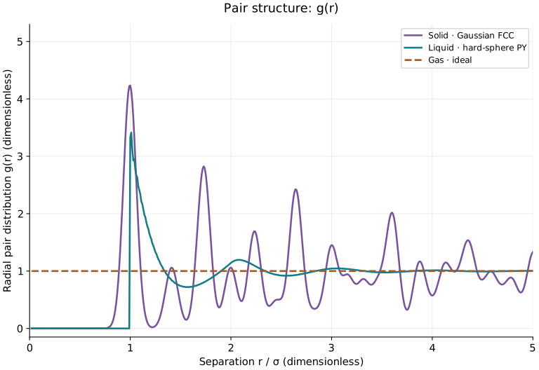
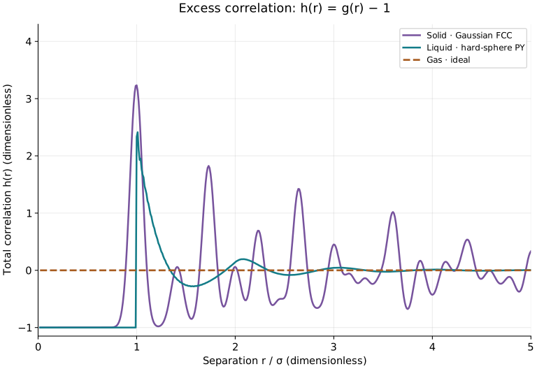
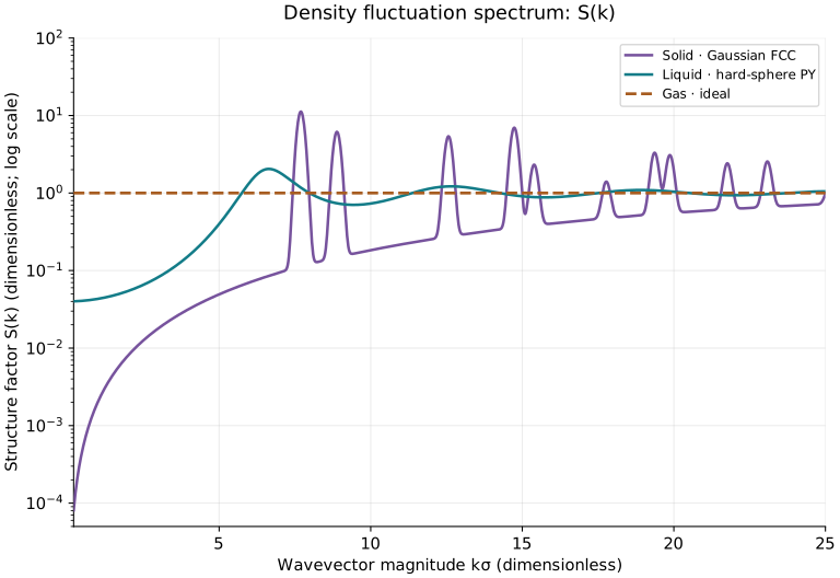
The same colors identify each reference model in all three plots. σ is a reference length: the liquid hard-sphere diameter and the solid nearest-neighbor lattice spacing. All functions are dimensionless; S(k) uses a logarithmic vertical axis so both low-k suppression and sharp peaks remain visible.
Models, parameters, and how the curves were calculated
- Gas: ideal uncorrelated classical particles: g(r)=1, h(r)=0, S(k)=1 at nonzero wavevector.
- Liquid: three-dimensional monodisperse hard spheres at packing fraction φ=0.40, nσ³=6φ/π≈0.76394. The Percus–Yevick direct-correlation polynomial is Fourier-transformed, then S=1/(1−nĉ). The radial inverse of S−1 gives h outside the core. g=0 for r<σ and the exact PY right-contact value g(σ+)=3.33333 are imposed at the discontinuity. Inversion uses kmaxσ=400 and Δkσ=0.05; small truncation oscillations remain near contact.
- Solid: an FCC point lattice with independent isotropic Gaussian displacements of standard deviation 0.045σ per Cartesian coordinate; nσ³=√2. Radial g is the powder average of Gaussian relative-displacement distributions summed over lattice neighbors. h is exactly g−1. This harmonic reference allows arbitrarily close pairs with extremely small probability; it is not a hard-sphere solid.
- Crystal S(k): diffuse scattering 1−exp(−k²s²), plus FCC reciprocal-lattice Bragg shells weighted by exp(−G²s²). Each radial delta peak is replaced by an area-normalized Gaussian of width 0.12 in kσ for display. The intensity includes elastic Bragg scattering; the uniform forward peak at k=0 is excluded. It is not the connected fluctuation spectrum about a fixed periodic mean density.
The curves use different densities and statistical models. They illustrate order, not a single material at one temperature or a simulated phase-change trajectory. The solid is powder-averaged; a single crystal has direction-dependent diffraction. Do not apply the homogeneous-liquid compressibility formula to the displayed crystal Bragg spectrum, or infer pressure from a peak height. The display-broadened crystal S is not an exact inverse transform of the unsmoothed radial g shown here.
SasView: PY hard-sphere reference ↗ · LAMMPS: crystalline diffraction definitions ↗
Reproducible plot data: g(r) and h(r) CSV · S(k) CSV · All data and parameters (JSON)
1. Factorize the dilute-gas partition function
- Neglect interparticle potential energy for an ideal monatomic gas. The position integral gives V^N and the Gaussian momentum integral supplies the thermal wavelength.
- Apply Stirling’s approximation to ln(N!) in the thermodynamic limit to obtain F.
- Differentiate F with respect to V for pressure; average three translational quadratic degrees of freedom for U.
Connection / worked consequence. Worked example: N=10²³ particles, V=0.01 m³, T=300 K give p=41,419.47 Pa and U=621.292 J. These are ideal monatomic estimates, not universal gas properties.
↑ Return to the state pathway2. From correlated particles to binary collisions
- Start from the reduced-distribution hierarchy on the overview page. Resolve encounters as brief, isolated binary collisions between long free flights.
- Approximate incoming two-particle velocity statistics by a product of one-particle distributions: molecular chaos.
- Count gain and loss into a velocity element using the differential cross-section, relative speed, and collision kinematics. For reversible elastic collisions the primed variables can label the corresponding inverse process.
Connection / worked consequence. Conservation of particle number, momentum, and energy in each elastic collision produces the corresponding collision-integral invariants.
↑ Return to the state pathway3. Velocity moments produce fluid balance laws
- Integrate the kinetic equation over velocity; the number-conserving collision integral vanishes, giving continuity.
- Multiply by m v and integrate. Separate bulk motion from peculiar velocity to obtain momentum balance and the pressure tensor.
- A local Maxwellian gives P=pI and Euler-level closure. For small Knudsen number and near local equilibrium, a first-order Chapman-Enskog treatment generates viscosity and thermal conductivity for Navier-Stokes-Fourier.
Connection / worked consequence. Large Kn, strong nonequilibrium, or sharp layers can require Boltzmann or DSMC rather than conventional continuum closure.
↑ Return to the state pathway4. Gas → plasma: add reaction equilibrium or kinetics
- Allow ionization to change the populations of neutral atoms, ions, and electrons while conserving nuclei and charge.
- For local thermodynamic equilibrium, equate the reaction chemical potentials and use ideal nondegenerate translational partition functions.
- Separate the ionization energy χ and internal partition functions U0, Ui; the free-electron spin factor gives the displayed Saha relation. Away from equilibrium, use ionization/recombination rate equations instead.
Connection / worked consequence. Ionization can be partial and gradual. A plasma also requires collective electromagnetic behavior on the scales of interest; it is not defined by a single universal temperature.
↑ Return to the state pathwayRelated models & worked graphical examples
These entries come from the existing catalog. Open a formulation here, or follow its link for the complete model and three worked examples.
Ideal gas equation of state
Relates pressure, volume and temperature for a dilute noninteracting gas.
Assumptions. n is amount in moles, V volume and T absolute temperature; intermolecular interactions and finite molecular volume are neglected.
Application. Estimating the amount of air in a low-pressure vessel.
Full model, derivation, references, numerical techniques & 3 worked graphs ↗Van der Waals equation of state
Adds molecular attraction and excluded volume to an ideal gas model.
Assumptions. v is molar volume; a and b are substance parameters. This is a qualitative equation of state near critical and coexistence regions.
Application. Qualitative liquid-vapor coexistence.
Full model, derivation, references, numerical techniques & 3 worked graphs ↗Virial equation of state
Represents nonideal behavior as a density or pressure expansion.
Assumptions. B and C are temperature-dependent molar virial coefficients; this low-density expansion may converge poorly near condensation.
Application. Gas properties away from the dilute limit.
Full model, derivation, references, numerical techniques & 3 worked graphs ↗Navier–Stokes model
Conserves mass and momentum for a viscous continuum fluid.
Assumptions. u is velocity, p pressure, ρ density and μ dynamic viscosity. Compressible flow also needs energy and an equation of state.
Application. Water flow around a valve.
Full model, derivation, references, numerical techniques & 3 worked graphs ↗Euler flow model
Neglects viscous stresses in compressible or incompressible flow.
Assumptions. D/Dt = ∂t+u·∇ is the material derivative. Inviscid approximations do not reproduce no-slip wall layers.
Application. First estimates of inviscid aerodynamic behavior.
Full model, derivation, references, numerical techniques & 3 worked graphs ↗Boltzmann kinetic equation
Evolves a particle distribution under transport and collisions.
Assumptions. Boltzmann kinetic equation; collision assumptions, molecular interaction laws and closure determine C[f].
Application. Gas kinetics outside simple continuum conditions.
Full model, derivation, references, numerical techniques & 3 worked graphs ↗Direct simulation Monte Carlo (DSMC)
Samples particle motion and collisions in a rarefied gas.
Assumptions. DSMC acceptance also depends on particle statistical weights and collision-selection scheme; cell/time scales must resolve mean-free-path and collision-time behavior.
Application. Gas flow where continuum assumptions fail.
Full model, derivation, references, numerical techniques & 3 worked graphs ↗Notation used throughout
n: number density (m⁻³); N: particle count; ρ: mass density (kg m⁻³); ρc: charge density; p: pressure; T: temperature (K); kB: Boltzmann constant; h, ℏ: Planck constants; β=1/(kBT); μ: chemical potential; f: phase-space distribution; g(r): pair distribution. In solid displacements u is a displacement; in the liquid closure u(r) is pair energy; in fluid equations u is bulk velocity. Subscripts identify phase or species. Every approximation must use consistent SI units or explicitly stated reduced units.