PHYSICS / ENGINEERING / COMPUTING
Particle unification: established theory and open proposals
Derive the gauge-theory framework, electroweak mixing and running couplings, then examine what grand unification and quantum gravity would need to explain.
Matter pathway: atom → solid → liquid → gas → plasma. Quantum mechanics and quantum field theory provide foundations across the pathway; they are not additional phases. This is a connected modeling route, not a universal heating curve. Actual phases depend on pressure, composition, and kinetics.
1. Gauge symmetry and the Standard Model
Definitions & inputs. g coupling,T generators,Aμ gauge fields,ψ matter field,Fμν field strength.
A gauge connection compensates local changes of the matter-field basis.
The commutator defines field strength including non-Abelian self-interactions.
Gauge, matter, Higgs and Yukawa terms form the schematic structure.
Interpretation. The Standard Model uses SU(3)c×SU(2)L×U(1)Y, a product group rather than a single simple grand-unified gauge group. Gravity is not included.
↑ Return to definitions and contents2. Electroweak mixing and masses
Definitions & inputs. g weakSU2 coupling,gprime hypercharge coupling,v Higgs expectation value,θW weak angle.
Insert the Higgs expectation value into its kinetic term to obtain the neutral gauge mass matrix.
Rotate into the massless photon and massive neutral boson.
Diagonalization fixes the tree-level mixing and masses; the photon remains massless.
Interpretation. Electroweak unification does not imply electromagnetism and the weak force have equal low-energy behavior.
↑ Return to definitions and contents3. Running couplings and grand unification
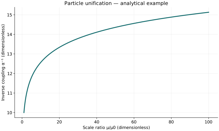
Definitions & inputs. αi=gi²/(4π),bi one-loop coefficients,μ renormalization scale,Λ candidate unification scale.
Quantum corrections change effective couplings with scale under this sign convention.
Differentiate1/α and integrate whilebi stays fixed.
A pairwise crossing can be solved algebraically; all relevant couplings and thresholds must agree for a unification claim.
Interpretation. SU5, SO10 and related proposals embed gauge and matter representations. A crossing alone does not establish a GUT; proton decay, neutrinos, symmetry breaking and threshold corrections are independent tests.
↑ Return to definitions and contents4. Effective operators, neutrinos and gravity
Definitions & inputs. Λ heavy scale,Od operator of mass dimension d,cd dimensionless coefficient,GFermi gravitational Newton constant G in Planck definitions.
Symmetries organize possible effects of unresolved high-energy degrees of freedom.
A simple heavy-neutrino seesaw and dimension-six decay scaling illustrate distinct potential probes, not universal predictions.
Dimensional combinations identify a scale at which quantum gravitational effects may be important; they do not derive a theory of everything.
Interpretation. String theory seeks quantum gravity with additional consistency structure; loop quantum gravity quantizes geometric degrees of freedom and is not by itself a particle GUT; asymptotic safety studies ultraviolet fixed points. None should be labeled experimentally confirmed unification.
↑ Return to definitions and contentsGraphical worked example
Twenty worked examples
Open a problem to see its defined inputs, assumptions, equation, numerical substitution, result, and interpretation. Values are illustrative analytical exercises.
Example 01. SU2 generator count
Definitions & inputs. n2.
Choose the governing model and isolate the requested quantity.
Insert the stated inputs in consistent units or the explicitly defined normalized units.
Evaluate the expression; the result uses the units shown.
Interpretation. Gauge algebra count.
↑ Return to definitions and contentsExample 02. SU3 generator count
Definitions & inputs. n3.
Choose the governing model and isolate the requested quantity.
Insert the stated inputs in consistent units or the explicitly defined normalized units.
Evaluate the expression; the result uses the units shown.
Interpretation. Eight gluon gauge fields.
↑ Return to definitions and contentsExample 03. Standard Model gauge count
Definitions & inputs. SU3,SU2,U1.
Choose the governing model and isolate the requested quantity.
Insert the stated inputs in consistent units or the explicitly defined normalized units.
Evaluate the expression; the result uses the units shown.
Interpretation. Before symmetry-breaking field rotation.
↑ Return to definitions and contentsExample 04. SU5 generator count
Definitions & inputs. n5.
Choose the governing model and isolate the requested quantity.
Insert the stated inputs in consistent units or the explicitly defined normalized units.
Evaluate the expression; the result uses the units shown.
Interpretation. Hypothetical gauge embedding.
↑ Return to definitions and contentsExample 05. ExtraSU5 generators
Definitions & inputs. 24minus12SM.
Choose the governing model and isolate the requested quantity.
Insert the stated inputs in consistent units or the explicitly defined normalized units.
Evaluate the expression; the result uses the units shown.
Interpretation. Counting alone does not specify their masses.
↑ Return to definitions and contentsExample 06. SO10 generator count
Definitions & inputs. n10.
Choose the governing model and isolate the requested quantity.
Insert the stated inputs in consistent units or the explicitly defined normalized units.
Evaluate the expression; the result uses the units shown.
Interpretation. Lie algebra dimension.
↑ Return to definitions and contentsExample 07. Electron charge
Definitions & inputs. Left lepton T3−.5,Y−.5.
Choose the governing model and isolate the requested quantity.
Insert the stated inputs in consistent units or the explicitly defined normalized units.
Evaluate the expression; the result uses the units shown.
Interpretation. Charge in units of positive e.
↑ Return to definitions and contentsExample 08. Neutrino charge
Definitions & inputs. T3+.5,Y−.5.
Choose the governing model and isolate the requested quantity.
Insert the stated inputs in consistent units or the explicitly defined normalized units.
Evaluate the expression; the result uses the units shown.
Interpretation. Same hypercharge doublet.
↑ Return to definitions and contentsExample 09. Up-quark charge
Definitions & inputs. T3+.5,Y1/6.
Choose the governing model and isolate the requested quantity.
Insert the stated inputs in consistent units or the explicitly defined normalized units.
Evaluate the expression; the result uses the units shown.
Interpretation. Left quark doublet convention.
↑ Return to definitions and contentsExample 10. Down-quark charge
Definitions & inputs. T3−.5,Y1/6.
Choose the governing model and isolate the requested quantity.
Insert the stated inputs in consistent units or the explicitly defined normalized units.
Evaluate the expression; the result uses the units shown.
Interpretation. Same convention.
↑ Return to definitions and contentsExample 11. Weak angle
Definitions & inputs. Illustrative g.65,gprime.36.
Choose the governing model and isolate the requested quantity.
Insert the stated inputs in consistent units or the explicitly defined normalized units.
Evaluate the expression; the result uses the units shown.
Interpretation. Tree-level toy inputs.
↑ Return to definitions and contentsExample 12. Electromagnetic coupling
Definitions & inputs. Same couplings.
Choose the governing model and isolate the requested quantity.
Insert the stated inputs in consistent units or the explicitly defined normalized units.
Evaluate the expression; the result uses the units shown.
Interpretation. Natural-unit coupling.
↑ Return to definitions and contentsExample 13. W mass
Definitions & inputs. g.65,v246GeV.
Choose the governing model and isolate the requested quantity.
Insert the stated inputs in consistent units or the explicitly defined normalized units.
Evaluate the expression; the result uses the units shown.
Interpretation. Tree-level exercise, not a precision mass prediction.
↑ Return to definitions and contentsExample 14. Z mass
Definitions & inputs. g.65,gprime.36,v246GeV.
Choose the governing model and isolate the requested quantity.
Insert the stated inputs in consistent units or the explicitly defined normalized units.
Evaluate the expression; the result uses the units shown.
Interpretation. Same illustrative inputs.
↑ Return to definitions and contentsExample 15. Tree mass ratio
Definitions & inputs. Same couplings.
Choose the governing model and isolate the requested quantity.
Insert the stated inputs in consistent units or the explicitly defined normalized units.
Evaluate the expression; the result uses the units shown.
Interpretation. Equals cosθW at tree level.
↑ Return to definitions and contentsExample 16. Hypercharge normalization
Definitions & inputs. αY.01.
Choose the governing model and isolate the requested quantity.
Insert the stated inputs in consistent units or the explicitly defined normalized units.
Evaluate the expression; the result uses the units shown.
Interpretation. Conventional SU5 normalization.
↑ Return to definitions and contentsExample 17. One-loop inverse coupling
Definitions & inputs. αinv0=10,b=−7,μ/μ0=10.
Choose the governing model and isolate the requested quantity.
Insert the stated inputs in consistent units or the explicitly defined normalized units.
Evaluate the expression; the result uses the units shown.
Interpretation. Fixed field content and sign convention.
↑ Return to definitions and contentsExample 18. Dimension-six amplitude suppression
Definitions & inputs. E100GeV,Λ10000GeV,c1.
Choose the governing model and isolate the requested quantity.
Insert the stated inputs in consistent units or the explicitly defined normalized units.
Evaluate the expression; the result uses the units shown.
Interpretation. Scaling only; matrix elements can change observable effects.
↑ Return to definitions and contentsExample 19. Seesaw mass scale
Definitions & inputs. y.1,v246GeV,M10¹⁴GeV.
Choose the governing model and isolate the requested quantity.
Insert the stated inputs in consistent units or the explicitly defined normalized units.
Evaluate the expression; the result uses the units shown.
Interpretation. GeV converted toeV; one-generation illustrative heavy-neutrino model.
↑ Return to definitions and contentsExample 20. Decay lifetime scaling
Definitions & inputs. Increase heavyΛby factor2,all other parameters fixed.
Choose the governing model and isolate the requested quantity.
Insert the stated inputs in consistent units or the explicitly defined normalized units.
Evaluate the expression; the result uses the units shown.
Interpretation. Dimension-six scaling; no numerical proton lifetime is inferred.
↑ Return to definitions and contentsSymbols and units
Each derivation and problem defines its own symbols and inputs. Symbols may be reused with different meanings in other subjects. Keep units consistent, retain sufficient precision during calculation, and apply the stated validity limits.