PHYSICS / ENGINEERING / COMPUTING
Electric car and motor design
Connect road loads to battery energy, inverter power, motor torque, regeneration and thermal management.
Matter pathway: atom → solid → liquid → gas → plasma. Quantum mechanics and quantum field theory provide foundations across the pathway; they are not additional phases. This is a connected modeling route, not a universal heating curve. Actual phases depend on pressure, composition, and kinetics.
1. Battery and vehicle energy
Definitions & inputs. Eusable battery energy,e consumption per distance,η charging efficiency,Vpack voltage,Ah charge capacity.
Volts times ampere-hours gives watt-hours, then apply the usable fraction.
Divide available energy by a defined driving-cycle consumption.
Distinguish grid energy from energy stored in the pack.
Interpretation. Range is not a fixed battery property; speed, weather, HVAC, tires and terrain change consumption.
↑ Return to definitions and contents2. Motor torque and field interaction
Definitions & inputs. B flux density,I current,l conductor length,kt torque constant,ke back EMF constant,ω speed.
Lorentz force on a perpendicular conductor is the elementary torque mechanism.
Winding voltage pays for resistance, inductive change and motion-induced EMF.
Separate shaft power from copper loss.
Interpretation. Permanent-magnet synchronous, induction and reluctance machines have different field production and control; this equivalent model is not universal.
↑ Return to definitions and contents3. Synchronous-machine dq model
Definitions & inputs. p pole pairs,ψf magnet flux linkage,id andiq currents,Ld andLq inductances,ωe electrical speed.
Magnet and reluctance contributions combine in electromagnetic torque.
Rotation couples the d-axis voltage to q-axis flux.
BackEMF and cross-coupling consume inverter voltage headroom.
Interpretation. Field weakening, current limits and voltage ellipse constrain high speed operation; control loop delay and rotor position accuracy matter.
↑ Return to definitions and contents4. Regeneration and thermal limits
Definitions & inputs. K vehicle kinetic energy,ηregen net recovery fraction,Rth thermal resistance,Cth thermal capacitance.
Recover only part of the reduction in kinetic energy, subject to power and traction limits.
Stored heat and cooling determine component temperature.
Steady rise and transient timescale follow from the thermal ODE.
Interpretation. Inverter loss, iron loss, bearing loss, pack heat and coolant power are additional parts of vehicle efficiency.
↑ Return to definitions and contentsGraphical worked example
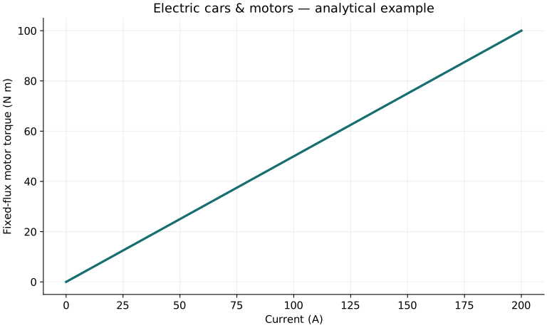
Twenty worked examples
Open a problem to see its defined inputs, assumptions, equation, numerical substitution, result, and interpretation. Values are illustrative analytical exercises.
Example 01. Nominal pack energy
Definitions & inputs. V400V,capacity150Ah.
Choose the governing model and isolate the requested quantity.
Insert the stated inputs in consistent units or the explicitly defined normalized units.
Evaluate the expression; the result uses the units shown.
Interpretation. Nominal voltage approximation.
↑ Return to definitions and contentsExample 02. Usable energy
Definitions & inputs. Nominal60kWh,f.9.
Choose the governing model and isolate the requested quantity.
Insert the stated inputs in consistent units or the explicitly defined normalized units.
Evaluate the expression; the result uses the units shown.
Interpretation. Excludes reserve by definition.
↑ Return to definitions and contentsExample 03. Cycle range
Definitions & inputs. Eu54kWh,consumption.18kWh/km.
Choose the governing model and isolate the requested quantity.
Insert the stated inputs in consistent units or the explicitly defined normalized units.
Evaluate the expression; the result uses the units shown.
Interpretation. Defined cycle only.
↑ Return to definitions and contentsExample 04. Charging input
Definitions & inputs. Store54kWh,η.9.
Choose the governing model and isolate the requested quantity.
Insert the stated inputs in consistent units or the explicitly defined normalized units.
Evaluate the expression; the result uses the units shown.
Interpretation. Includes assumed charge conversion loss.
↑ Return to definitions and contentsExample 05. Ideal constant-power charge time
Definitions & inputs. Energy30kWh,power50kW.
Choose the governing model and isolate the requested quantity.
Insert the stated inputs in consistent units or the explicitly defined normalized units.
Evaluate the expression; the result uses the units shown.
Interpretation. Real charging typically tapers.
↑ Return to definitions and contentsExample 06. Pack current
Definitions & inputs. DCpower40kW,V400V.
Choose the governing model and isolate the requested quantity.
Insert the stated inputs in consistent units or the explicitly defined normalized units.
Evaluate the expression; the result uses the units shown.
Interpretation. Ignore voltage sag in this step.
↑ Return to definitions and contentsExample 07. Series cells
Definitions & inputs. Cell nominal3.7V,target approximately400V,108cells.
Choose the governing model and isolate the requested quantity.
Insert the stated inputs in consistent units or the explicitly defined normalized units.
Evaluate the expression; the result uses the units shown.
Interpretation. Integer cell count gives nominal pack voltage.
↑ Return to definitions and contentsExample 08. Parallel capacity
Definitions & inputs. Cell5Ah,30parallel.
Choose the governing model and isolate the requested quantity.
Insert the stated inputs in consistent units or the explicitly defined normalized units.
Evaluate the expression; the result uses the units shown.
Interpretation. Matched cells and appropriate balancing.
↑ Return to definitions and contentsExample 09. DC-equivalent torque
Definitions & inputs. kt.5Nm/A,I100A.
Choose the governing model and isolate the requested quantity.
Insert the stated inputs in consistent units or the explicitly defined normalized units.
Evaluate the expression; the result uses the units shown.
Interpretation. Fixed flux and linear regime.
↑ Return to definitions and contentsExample 10. Back EMF
Definitions & inputs. ke.5Vs/rad,ω300rad/s.
Choose the governing model and isolate the requested quantity.
Insert the stated inputs in consistent units or the explicitly defined normalized units.
Evaluate the expression; the result uses the units shown.
Interpretation. Consistent SI constant.
↑ Return to definitions and contentsExample 11. Copper loss
Definitions & inputs. I100A,R.05Ω.
Choose the governing model and isolate the requested quantity.
Insert the stated inputs in consistent units or the explicitly defined normalized units.
Evaluate the expression; the result uses the units shown.
Interpretation. Equivalent winding resistance convention.
↑ Return to definitions and contentsExample 12. Mechanical power
Definitions & inputs. T50Nm,ω300rad/s.
Choose the governing model and isolate the requested quantity.
Insert the stated inputs in consistent units or the explicitly defined normalized units.
Evaluate the expression; the result uses the units shown.
Interpretation. Shaft torque definition.
↑ Return to definitions and contentsExample 13. Motor efficiency
Definitions & inputs. Pout15kW,loss1kW.
Choose the governing model and isolate the requested quantity.
Insert the stated inputs in consistent units or the explicitly defined normalized units.
Evaluate the expression; the result uses the units shown.
Interpretation. All relevant losses assumed included.
↑ Return to definitions and contentsExample 14. Electrical frequency
Definitions & inputs. p4pairs,shaft3000rpm.
Choose the governing model and isolate the requested quantity.
Insert the stated inputs in consistent units or the explicitly defined normalized units.
Evaluate the expression; the result uses the units shown.
Interpretation. Synchronous machine.
↑ Return to definitions and contentsExample 15. Surface-PM torque
Definitions & inputs. p4,ψf.1Wb,iq100A,Ld=Lq.
Choose the governing model and isolate the requested quantity.
Insert the stated inputs in consistent units or the explicitly defined normalized units.
Evaluate the expression; the result uses the units shown.
Interpretation. Specified peak dq convention.
↑ Return to definitions and contentsExample 16. Regenerated energy
Definitions & inputs. m1800kg,V20→0m/s,η.7.
Choose the governing model and isolate the requested quantity.
Insert the stated inputs in consistent units or the explicitly defined normalized units.
Evaluate the expression; the result uses the units shown.
Interpretation. Brake power and battery acceptance ignored.
↑ Return to definitions and contentsExample 17. Recovered watt-hours
Definitions & inputs. E252000J.
Choose the governing model and isolate the requested quantity.
Insert the stated inputs in consistent units or the explicitly defined normalized units.
Evaluate the expression; the result uses the units shown.
Interpretation. Small compared with pack capacity.
↑ Return to definitions and contentsExample 18. Steady motor temperature rise
Definitions & inputs. Ploss1000W,Rth.03K/W.
Choose the governing model and isolate the requested quantity.
Insert the stated inputs in consistent units or the explicitly defined normalized units.
Evaluate the expression; the result uses the units shown.
Interpretation. Linear constant coolant temperature.
↑ Return to definitions and contentsExample 19. Thermal time constant
Definitions & inputs. Rth.03K/W,Cth10000J/K.
Choose the governing model and isolate the requested quantity.
Insert the stated inputs in consistent units or the explicitly defined normalized units.
Evaluate the expression; the result uses the units shown.
Interpretation. Single node approximation.
↑ Return to definitions and contentsExample 20. Road-to-pack power
Definitions & inputs. Wheel20kW,motorη.94,inverterη.97.
Choose the governing model and isolate the requested quantity.
Insert the stated inputs in consistent units or the explicitly defined normalized units.
Evaluate the expression; the result uses the units shown.
Interpretation. Gear and accessory losses not included.
↑ Return to definitions and contentsSymbols and units
Each derivation and problem defines its own symbols and inputs. Symbols may be reused with different meanings in other subjects. Keep units consistent, retain sufficient precision during calculation, and apply the stated validity limits.