CONNECTED PHYSICS / STATES OF MATTER
Solid-state physics
Ordered reference positions, small displacements, and quantum electronic states. Start with the microscopic Hamiltonian and keep the structure that makes a crystal a crystal.
Matter pathway: atom → solid → liquid → gas → plasma. Quantum mechanics and quantum field theory provide foundations across the pathway; they are not additional phases. This is a connected modeling route, not a universal heating curve. Actual phases depend on pressure, composition, and kinetics.
Jump to gas / liquid / solid comparison plots ↓
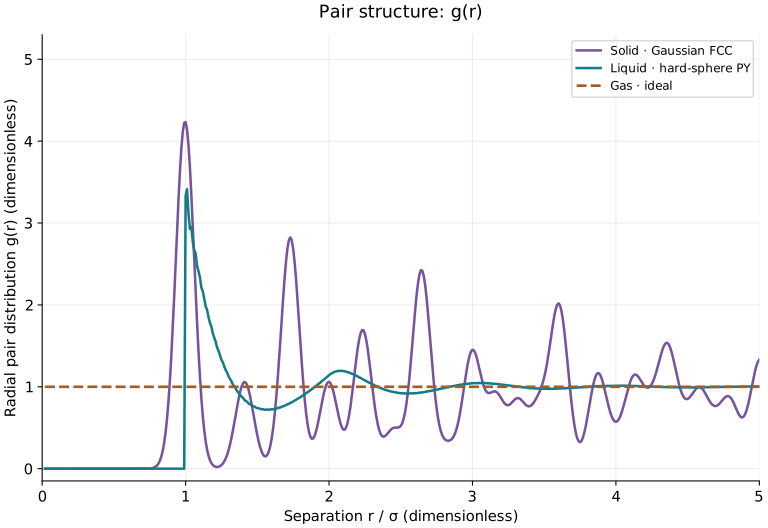
Compare gas, liquid, and solid structure
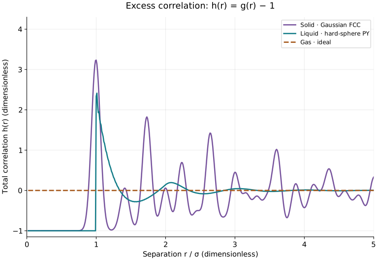
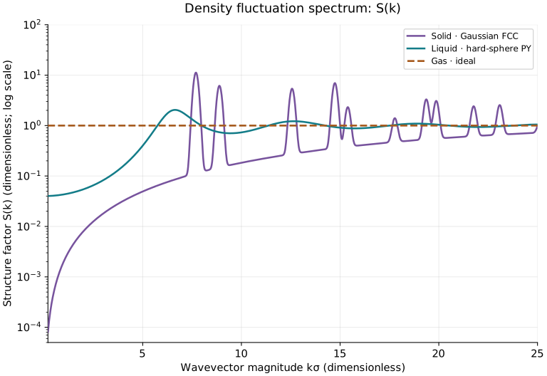
The same colors identify each reference model in all three plots. σ is a reference length: the liquid hard-sphere diameter and the solid nearest-neighbor lattice spacing. All functions are dimensionless; S(k) uses a logarithmic vertical axis so both low-k suppression and sharp peaks remain visible.
Models, parameters, and how the curves were calculated
- Gas: ideal uncorrelated classical particles: g(r)=1, h(r)=0, S(k)=1 at nonzero wavevector.
- Liquid: three-dimensional monodisperse hard spheres at packing fraction φ=0.40, nσ³=6φ/π≈0.76394. The Percus–Yevick direct-correlation polynomial is Fourier-transformed, then S=1/(1−nĉ). The radial inverse of S−1 gives h outside the core. g=0 for r<σ and the exact PY right-contact value g(σ+)=3.33333 are imposed at the discontinuity. Inversion uses kmaxσ=400 and Δkσ=0.05; small truncation oscillations remain near contact.
- Solid: an FCC point lattice with independent isotropic Gaussian displacements of standard deviation 0.045σ per Cartesian coordinate; nσ³=√2. Radial g is the powder average of Gaussian relative-displacement distributions summed over lattice neighbors. h is exactly g−1. This harmonic reference allows arbitrarily close pairs with extremely small probability; it is not a hard-sphere solid.
- Crystal S(k): diffuse scattering 1−exp(−k²s²), plus FCC reciprocal-lattice Bragg shells weighted by exp(−G²s²). Each radial delta peak is replaced by an area-normalized Gaussian of width 0.12 in kσ for display. The intensity includes elastic Bragg scattering; the uniform forward peak at k=0 is excluded. It is not the connected fluctuation spectrum about a fixed periodic mean density.
The curves use different densities and statistical models. They illustrate order, not a single material at one temperature or a simulated phase-change trajectory. The solid is powder-averaged; a single crystal has direction-dependent diffraction. Do not apply the homogeneous-liquid compressibility formula to the displayed crystal Bragg spectrum, or infer pressure from a peak height. The display-broadened crystal S is not an exact inverse transform of the unsmoothed radial g shown here.
SasView: PY hard-sphere reference ↗ · LAMMPS: crystalline diffraction definitions ↗
Reproducible plot data: g(r) and h(r) CSV · S(k) CSV · All data and parameters (JSON)
1. Expand about a mechanically stable crystal
- Choose equilibrium lattice positions R where the first derivatives of U vanish.
- Taylor-expand the energy; the Hessian Φ contains second derivatives with respect to displacements.
- Drop cubic and higher terms. Differentiating the quadratic energy gives coupled linear oscillator equations.
Connection / worked consequence. Heating increases vibrational amplitudes. Once rearrangements become important, this local expansion no longer describes the liquid; simply raising T in a harmonic formula does not derive melting.
↑ Return to the state pathway2. Diagonalize the vibrations and count quantum excitations
- Fourier-transform lattice displacements and mass-weight the force constants to construct D(q).
- Each eigenmode becomes a harmonic oscillator. Apply Bose occupation to its vibrational energy.
- Differentiate at fixed volume. Equal frequencies give Einstein’s model; an acoustic density of states proportional to frequency squared, normalized to 3N modes, gives Debye’s model.
Connection / worked consequence. Worked limit: Debye gives CV/(NkB)≈(12π⁴/5)(T/ΘD)³. Doubling a sufficiently low temperature multiplies this lattice contribution by eight; it does not imply eight times the total heat capacity of a metal.
↑ Return to the state pathway3. Retain the crystal’s periodic electronic environment
- For a static periodic one-electron effective Hamiltonian, use translation symmetry to choose Bloch states with periodic u.
- A localized-orbital expansion leads to tight binding. Keeping one orbital and nearest-neighbor hopping gives the displayed one-dimensional cosine band.
- A weak periodic potential instead mixes nearly degenerate free plane waves; a two-state diagonalization opens a gap of 2|VG| at a Bragg plane.
Connection / worked consequence. Loss of crystalline order removes this simple Bloch description. Liquids still have electrons and interactions, but generally lack a fixed periodic lattice.
↑ Return to the state pathway4. Solid → liquid: replace a fixed lattice by statistical structure
- Compute or approximate consistent solid and liquid free energies, including relevant vibrational, configurational, and electronic contributions.
- At melting under specified pressure, compare Gibbs free energies. The stable phase has the smaller value; coexistence occurs when they are equal.
- For an isotropic homogeneous liquid, replace permanent lattice sites by a pair-distribution function g(r) describing the likelihood of separations.
Connection / worked consequence. Continue to the liquid page: interactions survive melting. The key modeling change is how positions and correlations are described.
↑ Return to the state pathwayRelated models & worked graphical examples
These entries come from the existing catalog. Open a formulation here, or follow its link for the complete model and three worked examples.
Density functional theory (DFT)
Uses electron density to determine ground-state properties with an approximate exchange-correlation functional.
Assumptions. fᵢ are orbital occupations. vxc = δExc/δn is approximated in practical calculations.
Application. Screening electrode materials.
Full model, derivation, references, numerical techniques & 3 worked graphs ↗Heisenberg spin model
Represents interacting localized magnetic moments.
Assumptions. Sᵢ are dimensionless spin operators; positive J favors parallel spins under this sign convention. g is the Landé factor and μB the Bohr magneton.
Application. Temperature-dependent magnetic ordering.
Full model, derivation, references, numerical techniques & 3 worked graphs ↗Ising model
Represents discrete spins with interaction energies.
Assumptions. J and h have energy units; dimensionality, interaction range and boundary conditions change the predicted behavior.
Application. Studying phase transitions in a simplified magnet.
Full model, derivation, references, numerical techniques & 3 worked graphs ↗Quantum harmonic oscillator
Describes a quantum degree of freedom in a quadratic potential.
Assumptions. n = 0,1,…; x measures displacement from equilibrium and ω is the natural frequency. Anharmonic terms are neglected.
Application. Approximating vibrational levels near equilibrium.
Full model, derivation, references, numerical techniques & 3 worked graphs ↗Einstein crystal heat-capacity model
Treats crystal vibrations as independent quantum oscillators at a single frequency.
Assumptions. Theta_E=hbar omega_E/k_B. Independent harmonic oscillators with one frequency; ignores dispersion, acoustic low-frequency modes, anharmonicity, and electronic heat capacity.
Application. Estimating an optical-mode contribution to crystal heat capacity.
Full model, derivation, references, numerical techniques & 3 worked graphs ↗Debye phonon model
Approximates acoustic phonons by a continuum spectrum with a mode-count cutoff.
Assumptions. Theta_D=hbar omega_D/k_B, N atom count. Isotropic harmonic continuum approximation with an effective sound speed; optical modes and anharmonic effects require extensions.
Application. Estimating low-temperature lattice heat capacity in crystalline solids.
Full model, derivation, references, numerical techniques & 3 worked graphs ↗Sommerfeld free-electron model
Describes conduction electrons as a degenerate, noninteracting Fermi gas.
Assumptions. N is electron count, n=N/V, T_F=E_F/k_B. Three-dimensional noninteracting spin-1/2 electrons with parabolic dispersion; the heat-capacity expression requires T much smaller than T_F.
Application. Estimating electronic heat capacity and Fermi energy in simple metals.
Full model, derivation, references, numerical techniques & 3 worked graphs ↗Tight-binding electronic model
Builds crystal electronic bands from localized orbitals and intersite hopping.
Assumptions. Displayed chain uses an orthonormal single orbital per site and real positive hopping t. Multiorbital materials require calibrated matrix elements and possibly overlap and spin-orbit coupling. Electron correlations are excluded unless added explicitly.
Application. Modeling semiconductor nanowire and crystalline-device electronic bands.
Full model, derivation, references, numerical techniques & 3 worked graphs ↗Nearly-free-electron model
Predicts band gaps by perturbing free electrons with a weak periodic potential.
Assumptions. epsilon_k=hbar²k²/(2m); a mean potential can be absorbed into the energy origin. Weak periodic potential, two-state approximation near a Bragg plane; remote states and strong correlations are omitted.
Application. Explaining Bragg-plane band gaps in weak-potential crystalline conductors.
Full model, derivation, references, numerical techniques & 3 worked graphs ↗Harmonic lattice dynamics
Computes phonon modes from a quadratic expansion of crystal potential energy.
Assumptions. D is the mass-weighted dynamical matrix; e is polarization, nu branch index. The displayed one-dimensional chain has nearest-neighbor spring constant K, mass m, and spacing a. Harmonic approximation excludes phonon scattering and thermal expansion.
Application. Predicting phonon dispersion, harmonic stability, and vibrational thermodynamics.
Full model, derivation, references, numerical techniques & 3 worked graphs ↗Notation used throughout
n: number density (m⁻³); N: particle count; ρ: mass density (kg m⁻³); ρc: charge density; p: pressure; T: temperature (K); kB: Boltzmann constant; h, ℏ: Planck constants; β=1/(kBT); μ: chemical potential; f: phase-space distribution; g(r): pair distribution. In solid displacements u is a displacement; in the liquid closure u(r) is pair energy; in fluid equations u is bulk velocity. Subscripts identify phase or species. Every approximation must use consistent SI units or explicitly stated reduced units.