PHYSICS / ENGINEERING / COMPUTING
Astrodynamics and orbital mechanics
Derive two-body trajectories, orbital elements, maneuver budgets, and relative-motion scales through twenty worked problems.
Matter pathway: atom → solid → liquid → gas → plasma. Quantum mechanics and quantum field theory provide foundations across the pathway; they are not additional phases. This is a connected modeling route, not a universal heating curve. Actual phases depend on pressure, composition, and kinetics.
1. Two-body energy and angular momentum
Definitions & inputs. r radius, v speed, μ=G(M+m), ε specific orbital energy, h specific angular momentum, a semimajor axis.
Newton’s central force governs the relative position.
Energy and angular momentum are conserved.
Rearrange conserved energy for vis-viva and use conic geometry.
Interpretation. Negative energy indicates a bound ellipse; positive energy indicates a hyperbola.
↑ Return to definitions and contents2. Orbital geometry and timing
Definitions & inputs. e eccentricity, E eccentric anomaly, M mean anomaly, ν true anomaly, n mean motion.
Periapsis and apoapsis are measured from the central body’s centre.
Kepler’s third law fixes the orbital period.
Equal-area motion leads to Kepler’s equation, usually solved numerically for E.
Interpretation. Altitude is radius minus the body radius; confusing them produces large errors.
↑ Return to definitions and contents3. Impulsive transfers and plane changes
Definitions & inputs. r1,r2 are circular-orbit radii; at=(r1+r2)/2; Δi is the angle between orbital planes.
Compare transfer periapsis speed with the initial circular speed.
Compare the final circular speed with transfer apoapsis speed for an outward transfer.
Transfer duration is half an ellipse; a pure plane change is the difference between two equal-length velocity vectors.
Interpretation. Combine maneuvers carefully; separately adding ideal burns can overestimate an optimized combined maneuver.
↑ Return to definitions and contents4. Relative motion and secular perturbations
Definitions & inputs. x radial and y along-track relative coordinates; J2 oblateness coefficient; i inclination.
Linearize central gravity in the rotating circular-orbit frame.
Differentiate n∝a⁻³/² for nearby orbits.
Oblateness produces a secular node drift; polar orbits have zero leading nodal drift.
Interpretation. Real orbit determination and mission planning need perturbations, covariance, epochs, and coordinate-frame definitions.
↑ Return to definitions and contentsGraphical worked example
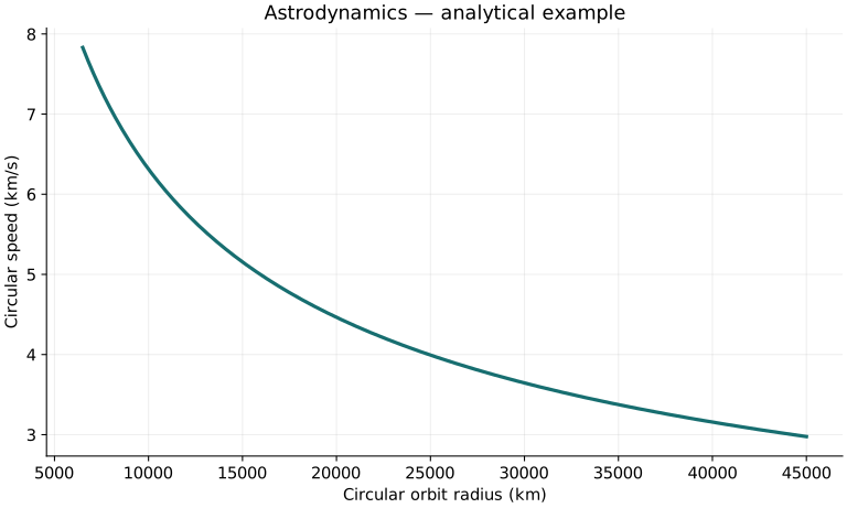
Twenty worked examples
Open a problem to see its defined inputs, assumptions, equation, numerical substitution, result, and interpretation. Values are illustrative analytical exercises.
Example 01. Orbit radius from altitude
Definitions & inputs. h=500 km, RE=6371 km.
Choose the governing model and isolate the requested quantity.
Insert the stated inputs in consistent units or the explicitly defined normalized units.
Evaluate the expression; the result uses the units shown.
Interpretation. Gravity formulas use radius from the centre.
↑ Return to definitions and contentsExample 02. Circular speed at 500 km
Definitions & inputs. r=6871000 m, μ=3.986004418×10¹⁴ SI.
Choose the governing model and isolate the requested quantity.
Insert the stated inputs in consistent units or the explicitly defined normalized units.
Evaluate the expression; the result uses the units shown.
Interpretation. Speed is relative to an inertial two-body frame.
↑ Return to definitions and contentsExample 03. Circular period
Definitions & inputs. r=6871000 m.
Choose the governing model and isolate the requested quantity.
Insert the stated inputs in consistent units or the explicitly defined normalized units.
Evaluate the expression; the result uses the units shown.
Interpretation. This is about 94.5 minutes.
↑ Return to definitions and contentsExample 04. Specific orbital energy
Definitions & inputs. a=7000000 m.
Choose the governing model and isolate the requested quantity.
Insert the stated inputs in consistent units or the explicitly defined normalized units.
Evaluate the expression; the result uses the units shown.
Interpretation. The negative sign denotes a bound orbit.
↑ Return to definitions and contentsExample 05. Escape speed at radius
Definitions & inputs. r=7000000 m.
Choose the governing model and isolate the requested quantity.
Insert the stated inputs in consistent units or the explicitly defined normalized units.
Evaluate the expression; the result uses the units shown.
Interpretation. Escape threshold has zero specific energy.
↑ Return to definitions and contentsExample 06. Periapsis radius
Definitions & inputs. a=10000 km, e=0.2.
Choose the governing model and isolate the requested quantity.
Insert the stated inputs in consistent units or the explicitly defined normalized units.
Evaluate the expression; the result uses the units shown.
Interpretation. Subtract Earth radius to obtain altitude.
↑ Return to definitions and contentsExample 07. Apoapsis radius
Definitions & inputs. a=10000 km, e=0.2.
Choose the governing model and isolate the requested quantity.
Insert the stated inputs in consistent units or the explicitly defined normalized units.
Evaluate the expression; the result uses the units shown.
Interpretation. Apoapsis is the farthest orbital point.
↑ Return to definitions and contentsExample 08. Periapsis speed
Definitions & inputs. a=10000000 m, rp=8000000 m.
Choose the governing model and isolate the requested quantity.
Insert the stated inputs in consistent units or the explicitly defined normalized units.
Evaluate the expression; the result uses the units shown.
Interpretation. The orbital speed is larger at periapsis.
↑ Return to definitions and contentsExample 09. Eccentricity from apsides
Definitions & inputs. rp=8000 km, ra=12000 km.
Choose the governing model and isolate the requested quantity.
Insert the stated inputs in consistent units or the explicitly defined normalized units.
Evaluate the expression; the result uses the units shown.
Interpretation. The same distances imply a=10000 km.
↑ Return to definitions and contentsExample 10. Mean motion
Definitions & inputs. a=7000000 m.
Choose the governing model and isolate the requested quantity.
Insert the stated inputs in consistent units or the explicitly defined normalized units.
Evaluate the expression; the result uses the units shown.
Interpretation. Mean anomaly advances uniformly in this model.
↑ Return to definitions and contentsExample 11. Mean anomaly from eccentric anomaly
Definitions & inputs. E=π/2 rad, e=0.1.
Choose the governing model and isolate the requested quantity.
Insert the stated inputs in consistent units or the explicitly defined normalized units.
Evaluate the expression; the result uses the units shown.
Interpretation. True anomaly and mean anomaly are generally different.
↑ Return to definitions and contentsExample 12. Hohmann first burn
Definitions & inputs. r1=7000 km, r2=14000 km.
Choose the governing model and isolate the requested quantity.
Insert the stated inputs in consistent units or the explicitly defined normalized units.
Evaluate the expression; the result uses the units shown.
Interpretation. The first tangential burn raises apoapsis.
↑ Return to definitions and contentsExample 13. Hohmann second burn
Definitions & inputs. r1=7000 km, r2=14000 km.
Choose the governing model and isolate the requested quantity.
Insert the stated inputs in consistent units or the explicitly defined normalized units.
Evaluate the expression; the result uses the units shown.
Interpretation. The second burn circularizes at apoapsis.
↑ Return to definitions and contentsExample 14. Hohmann coast time
Definitions & inputs. Transfer a=10500 km.
Choose the governing model and isolate the requested quantity.
Insert the stated inputs in consistent units or the explicitly defined normalized units.
Evaluate the expression; the result uses the units shown.
Interpretation. Only half the transfer ellipse is traversed.
↑ Return to definitions and contentsExample 15. Ten-degree plane change
Definitions & inputs. v=7500 m/s; Δi=10°.
Choose the governing model and isolate the requested quantity.
Insert the stated inputs in consistent units or the explicitly defined normalized units.
Evaluate the expression; the result uses the units shown.
Interpretation. Plane changes are expensive at high speed.
↑ Return to definitions and contentsExample 16. Synchronous orbit radius
Definitions & inputs. Desired inertial period T=86164 s.
Choose the governing model and isolate the requested quantity.
Insert the stated inputs in consistent units or the explicitly defined normalized units.
Evaluate the expression; the result uses the units shown.
Interpretation. Geostationary also requires an equatorial, prograde, circular orbit.
↑ Return to definitions and contentsExample 17. Hyperbolic excess speed
Definitions & inputs. Specific energy ε=4.5×10⁶ J/kg.
Choose the governing model and isolate the requested quantity.
Insert the stated inputs in consistent units or the explicitly defined normalized units.
Evaluate the expression; the result uses the units shown.
Interpretation. This is asymptotic relative speed to the central body.
↑ Return to definitions and contentsExample 18. Specific angular momentum
Definitions & inputs. Circular r=7000000 m.
Choose the governing model and isolate the requested quantity.
Insert the stated inputs in consistent units or the explicitly defined normalized units.
Evaluate the expression; the result uses the units shown.
Interpretation. This is angular momentum per unit orbiting mass.
↑ Return to definitions and contentsExample 19. Nearby-orbit drift rate
Definitions & inputs. a=7000 km, Δa=1 km.
Choose the governing model and isolate the requested quantity.
Insert the stated inputs in consistent units or the explicitly defined normalized units.
Evaluate the expression; the result uses the units shown.
Interpretation. The higher orbit advances more slowly in mean anomaly.
↑ Return to definitions and contentsExample 20. Polar J2 nodal drift
Definitions & inputs. Inclination i=90°.
Choose the governing model and isolate the requested quantity.
Insert the stated inputs in consistent units or the explicitly defined normalized units.
Evaluate the expression; the result uses the units shown.
Interpretation. Other perturbations may still move the node.
↑ Return to definitions and contentsSymbols and units
Each derivation and problem defines its own symbols and inputs. Symbols may be reused with different meanings in other subjects. Keep units consistent, retain sufficient precision during calculation, and apply the stated validity limits.