PHYSICS / ENGINEERING / COMPUTING
Statistical physics: microstates to thermodynamics
Derive equilibrium ensembles, free energies, ideal gases, fluctuations and simple interacting models.
Matter pathway: atom → solid → liquid → gas → plasma. Quantum mechanics and quantum field theory provide foundations across the pathway; they are not additional phases. This is a connected modeling route, not a universal heating curve. Actual phases depend on pressure, composition, and kinetics.
1. Entropy and canonical probabilities
Definitions & inputs. Ω micro state count,pi probability,β1/(kBT),Ei micro state energy,Z partition function.
Equal probability counting and Gibbs entropy connect microscopic uncertainty to entropy.
Maximize entropy with normalization and mean energy constraints.
Lagrange multipliers give Bolt z mann weights and the normalize r.
Interpretation. βis fixed by the bath;degenerate energy levels contribute their multiplicity to Z.
↑ Return to definitions and contents2. Thermodynamic derivatives
Definitions & inputs. F Helmholtz free energy,U mean internal energy,P pressure,CV heat capacity.
Partition function summarizes equilibrium state counting.
Differentiate the appropriate potential to obtain observable s.
Asecondβderivative connects energy fluctuations to response.
Interpretation. A partition function must include consistent energy zeros and quantum state-counting normalization.
↑ Return to definitions and contents3. Classical ideal gas
Definitions & inputs. λth=h/√(2πmkBT),N particle count,Vvolume.
Independent one-particle integrals factorize;N!removes classical over counting.
Volume and temperature derivatives yield the ideal gas law and translational energy.
Equipartition assigns kB T/2to each quadratic velocity component.
Interpretation. Internal rotation,vibration,interactions and quantum degeneracy add corrections.
↑ Return to definitions and contents4. Interactions, correlations and criticality
Definitions & inputs. sij=±1 spins,J interaction energy,H external field energy,g(r) pair distribution.
Interactions favor correlations rather than independent Bolt z mann factors.
Pair forces correct the ideal gas pressure through structure.
Grand-canonical number fluctuations measure a response function.
Interpretation. Critical phenomena need correlation lengths and finite-size analysis;mean field and Monte Carlo methods have different errors.
↑ Return to definitions and contentsGraphical worked example
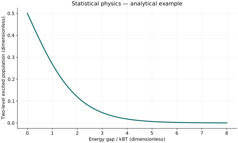
Twenty worked examples
Open a problem to see its defined inputs, assumptions, equation, numerical substitution, result, and interpretation. Values are illustrative analytical exercises.
Example 01. Entropy count
Definitions & inputs. Ω8.
Choose the governing model and isolate the requested quantity.
Insert the stated inputs in consistent units or the explicitly defined normalized units.
Evaluate the expression; the result uses the units shown.
Interpretation. Equal probability micro states.
↑ Return to definitions and contentsExample 02. Binary entropy
Definitions & inputs. p.5.
Choose the governing model and isolate the requested quantity.
Insert the stated inputs in consistent units or the explicitly defined normalized units.
Evaluate the expression; the result uses the units shown.
Interpretation. Natural-log entropy.
↑ Return to definitions and contentsExample 03. Thermal energy
Definitions & inputs. T300K,kB1.380649×10⁻²³SI.
Choose the governing model and isolate the requested quantity.
Insert the stated inputs in consistent units or the explicitly defined normalized units.
Evaluate the expression; the result uses the units shown.
Interpretation. Per-particle energy scale.
↑ Return to definitions and contentsExample 04. Boltzmann ratio
Definitions & inputs. Gap2kBT,equal degeneracy.
Choose the governing model and isolate the requested quantity.
Insert the stated inputs in consistent units or the explicitly defined normalized units.
Evaluate the expression; the result uses the units shown.
Interpretation. Two state weight ratio.
↑ Return to definitions and contentsExample 05. Two-level partition
Definitions & inputs. Levels0andΔ,kBT=Δ.
Choose the governing model and isolate the requested quantity.
Insert the stated inputs in consistent units or the explicitly defined normalized units.
Evaluate the expression; the result uses the units shown.
Interpretation. Non degenerate levels.
↑ Return to definitions and contentsExample 06. Excited population
Definitions & inputs. Same levels.
Choose the governing model and isolate the requested quantity.
Insert the stated inputs in consistent units or the explicitly defined normalized units.
Evaluate the expression; the result uses the units shown.
Interpretation. Normalized probability.
↑ Return to definitions and contentsExample 07. Mean energy
Definitions & inputs. Δ1eV,kBT1eV.
Choose the governing model and isolate the requested quantity.
Insert the stated inputs in consistent units or the explicitly defined normalized units.
Evaluate the expression; the result uses the units shown.
Interpretation. Two state canonical mean.
↑ Return to definitions and contentsExample 08. Two-level heat capacity
Definitions & inputs. xΔ/kBT=1.
Choose the governing model and isolate the requested quantity.
Insert the stated inputs in consistent units or the explicitly defined normalized units.
Evaluate the expression; the result uses the units shown.
Interpretation. Positive Sch ott ky response.
↑ Return to definitions and contentsExample 09. Free energy
Definitions & inputs. kBT1eV,Z1+exp−1.
Choose the governing model and isolate the requested quantity.
Insert the stated inputs in consistent units or the explicitly defined normalized units.
Evaluate the expression; the result uses the units shown.
Interpretation. Chosen ground energy zero.
↑ Return to definitions and contentsExample 10. Ideal-gas pressure
Definitions & inputs. n2.5×10²⁵/m³,T300K.
Choose the governing model and isolate the requested quantity.
Insert the stated inputs in consistent units or the explicitly defined normalized units.
Evaluate the expression; the result uses the units shown.
Interpretation. Dilute classical gas.
↑ Return to definitions and contentsExample 11. One-mole energy
Definitions & inputs. T300K,R8.314462618.
Choose the governing model and isolate the requested quantity.
Insert the stated inputs in consistent units or the explicitly defined normalized units.
Evaluate the expression; the result uses the units shown.
Interpretation. Monatomic translational energy.
↑ Return to definitions and contentsExample 12. Molar CV
Definitions & inputs. Monatomic ideal gas.
Choose the governing model and isolate the requested quantity.
Insert the stated inputs in consistent units or the explicitly defined normalized units.
Evaluate the expression; the result uses the units shown.
Interpretation. Internal excitation s absent.
↑ Return to definitions and contentsExample 13. Molar CP
Definitions & inputs. Samegas.
Choose the governing model and isolate the requested quantity.
Insert the stated inputs in consistent units or the explicitly defined normalized units.
Evaluate the expression; the result uses the units shown.
Interpretation. Ideal-gas identity.
↑ Return to definitions and contentsExample 14. Heat-capacity ratio
Definitions & inputs. Monatomic gas.
Choose the governing model and isolate the requested quantity.
Insert the stated inputs in consistent units or the explicitly defined normalized units.
Evaluate the expression; the result uses the units shown.
Interpretation. Classical translation only.
↑ Return to definitions and contentsExample 15. RMS speed
Definitions & inputs. m4.65×10⁻²⁶kg,T300K.
Choose the governing model and isolate the requested quantity.
Insert the stated inputs in consistent units or the explicitly defined normalized units.
Evaluate the expression; the result uses the units shown.
Interpretation. Translational Maxwell distribution.
↑ Return to definitions and contentsExample 16. Isothermal expansion entropy
Definitions & inputs. Onemole,V2/V1=2.
Choose the governing model and isolate the requested quantity.
Insert the stated inputs in consistent units or the explicitly defined normalized units.
Evaluate the expression; the result uses the units shown.
Interpretation. Ideal reversible end states.
↑ Return to definitions and contentsExample 17. Isothermal work
Definitions & inputs. Onemole300K,volume ratio2.
Choose the governing model and isolate the requested quantity.
Insert the stated inputs in consistent units or the explicitly defined normalized units.
Evaluate the expression; the result uses the units shown.
Interpretation. Work done by gas in reversible expansion.
↑ Return to definitions and contentsExample 18. Relative energy fluctuation
Definitions & inputs. N10⁶monatomic particles.
Choose the governing model and isolate the requested quantity.
Insert the stated inputs in consistent units or the explicitly defined normalized units.
Evaluate the expression; the result uses the units shown.
Interpretation. Canonical ideal-gas result.
↑ Return to definitions and contentsExample 19. Metropolis uphill acceptance
Definitions & inputs. ΔE=2kBT.
Choose the governing model and isolate the requested quantity.
Insert the stated inputs in consistent units or the explicitly defined normalized units.
Evaluate the expression; the result uses the units shown.
Interpretation. Symmetric proposal;auto correlation still matters.
↑ Return to definitions and contentsExample 20. Single Ising pair flip cost
Definitions & inputs. J1energy unit,no external field,aligned→antialigned.
Choose the governing model and isolate the requested quantity.
Insert the stated inputs in consistent units or the explicitly defined normalized units.
Evaluate the expression; the result uses the units shown.
Interpretation. One bond only,not the whole lattice.
↑ Return to definitions and contentsSymbols and units
Each derivation and problem defines its own symbols and inputs. Symbols may be reused with different meanings in other subjects. Keep units consistent, retain sufficient precision during calculation, and apply the stated validity limits.