Rocket design models

1. Derive the ideal rocket equation

Definitions & inputs. m is vehicle mass, ve effective exhaust velocity, g0=9.80665 m/s², Isp specific impulse.

1. Momentum conservation relates velocity gain to expelled vehicle mass.

   $$m\,dv=-v_e\,dm$$

2. Integrate over decreasing mass.

   $$\Delta v=\int_{m_f}^{m_0}v_e\frac{dm}{m}=v_e\ln(m_0/m_f)$$

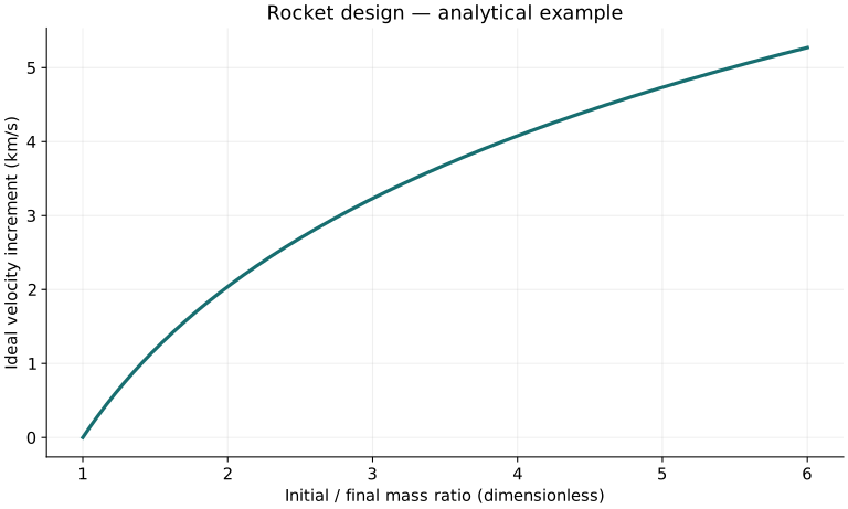
3. Specific impulse converts to effective velocity; required mass ratio grows exponentially.

   $$v_e=g_0I_{sp},\quad m_0/m_f=e^{\Delta v/(g_0I_{sp})}$$

Interpretation. Ideal Δv is not achieved orbital speed: gravity, drag, steering, and staging affect the trajectory.

• NASA Glenn — ideal rocket equation ↗

2. Thrust, flow, and impulse

Definitions & inputs. ṁ positive expelled mass rate, ue physical exhaust speed, pe exit pressure, pa ambient pressure, Ae exit area.

1. Momentum flux and pressure imbalance both contribute to thrust.

   $$F=\dot m u_e+(p_e-p_a)A_e$$

2. Specific impulse normalizes thrust by propellant weight flow; total impulse integrates force over time.

   $$I_{sp}=F/(\dot m g_0),\quad I_t=\int Fdt$$

3. Propellant allocation and mass flow set a simple burn duration.

   $$t_b=m_p/\dot m\quad(\dot m\ \text{constant})$$

Interpretation. Effective exhaust velocity includes pressure thrust and need not equal the physical exit speed.

• NASA Glenn — ideal rocket equation ↗

3. Force and energy budgets

Definitions & inputs. D aerodynamic drag, ρ air density, CD drag coefficient, A reference area, γ flight-path angle above horizontal.

1. Resolve forces along the instantaneous flight path.

   $$m\dot v=F-D-mg\sin\gamma$$

2. Dynamic pressure and drag require both atmospheric density and speed.

   $$q=\tfrac12\rho v^2,\quad D=qC_DA$$

3. Gravity loss depends on the trajectory, not simply burn duration in every case.

   $$\Delta v_{gravity}=\int g\sin\gamma\,dt$$

Interpretation. A rocket’s maximum dynamic pressure need not occur at maximum speed.

• NASA Glenn — ideal rocket equation ↗

4. Staging and thermal/mechanical estimates

Definitions & inputs. Each stage has its own ignition and burnout masses; η denotes conversion efficiency or a stated margin factor only in its local example.

1. Calculate each stage using the mass it accelerates, including upper stages and payload.

   $$\Delta v_{total}=\sum_i g_0I_{sp,i}\ln(m_{0,i}/m_{f,i})$$

2. Thrust-to-weight and average axial stress are distinct measures.

   $$\mathrm{TWR}=F/(mg_0),\quad\sigma=F/A$$

3. A lumped heat capacity gives a first estimate of temperature change.

   $$Q=mc_p\Delta T$$

Interpretation. Use consistent stage boundaries; do not multiply isolated stage mass ratios without accounting for discarded mass.

• NASA Glenn — ideal rocket equation ↗

5. Define Isp before comparing nuclear engines

Definitions & inputs. F is axial thrust, ṁp the explicitly counted consumed propellant mass rate, g0=9.80665 m/s², veff=F/ṁp effective exhaust speed, ηj jet efficiency, q fuel energy per kg, and f burned-fuel mass per kg of total consumed propellant. Specific impulse has units of seconds, not velocity.

1. Start from thrust. Effective exhaust speed equals actual gas speed only when the counted propellant and exhaust flow agree and pressure thrust is negligible.

   $$I_{sp}=\frac{F}{\dot m_p g_0}=\frac{v_{eff}}{g_0},\quad F=\dot m_e v_e+(p_e-p_a)A_e$$

2. For the stated simple material-exhaust model, convert a fraction of available reaction energy into directed kinetic power.

   $$P_{jet}=\tfrac12\dot m_p v_{eff}^2=\eta_j f\dot m_p q$$

3. Cancel the common mass-flow rate. Nuclear energy per kg of fuel alone does not fix Isp: ηj and fuel dilution f matter.

   $$v_{eff}\simeq\sqrt{2\eta_j f q},\quad I_{sp}\simeq\sqrt{2\eta_j f q}/g_0$$

4. At fixed jet power, raising exhaust speed lowers thrust. Check dimensions and check veff≪c before using the Newtonian energy formula.

   $$F=\frac{2P_{jet}}{v_{eff}},\quad [q]=\mathrm{J\,kg^{-1}}=\mathrm{m^2\,s^{-2}}$$

Interpretation. Fission thermal, fission electric, fusion-product and antimatter photon engines convert energy into momentum differently. The calculations below are idealized estimates under stated assumptions, not demonstrated ratings or reactor designs. The classical rocket equation also ceases to suffice when the vehicle becomes relativistic.

• NASA Glenn — Specific impulse ↗

6. Fission thermal propulsion: hot hydrogen sets the exhaust speed

Definitions & inputs. Tc is stagnation temperature, γ gas heat-capacity ratio, Ru=8.314462618 J/(mol K), M molar mass, pc and pe chamber and exit pressures, ηn fraction of ideal enthalpy drop converted to directed kinetic energy.

1. Apply a steady nozzle energy balance with kinetic-energy conversion efficiency ηn.

   $$c_p=\frac{\gamma}{\gamma-1}\frac{R_u}{M},\quad\frac{v_e^2}{2}=\eta_n c_p(T_c-T_e)$$

2. Use the isentropic ideal temperature drop as a reference and apply ηn to the available kinetic energy.

   $$\frac{T_e}{T_c}=\left(\frac{p_e}{p_c}\right)^{(\gamma-1)/\gamma}\Rightarrow v_e=\sqrt{\eta_n\frac{2\gamma}{\gamma-1}\frac{R_uT_c}{M}\left[1-\left(\frac{p_e}{p_c}\right)^{(\gamma-1)/\gamma}\right]}$$

3. Worked illustrative upper-expansion case: specify all thermodynamic assumptions rather than inferring exhaust velocity directly from fission energy.

   $$T_c=2800\,\mathrm K,\ M=0.002\,\mathrm{kg\,mol^{-1}},\ \gamma=1.4,\ \eta_n=0.90,\ p_e/p_c\to0$$

4. Evaluate the ideal-gas model, then divide by standard gravity. The zero exit-pressure limit is an ideal reference, not a finite-nozzle geometry.

   $$v_e=\sqrt{0.90(7)(8.314462618/0.002)(2800)}\simeq8563.5\,\mathrm{m\,s^{-1}},\quad I_{sp}\simeq873.2\,\mathrm s$$

Interpretation. This temperature-based estimate is the appropriate starting point for a nuclear thermal rocket. It must not be replaced by assuming all fission energy becomes kinetic energy of the reactor fuel itself. NASA’s NTP references discuss the underlying development and performance context.

• NASA — Nuclear thermal propulsion ↗

7. Fission electric propulsion: power, mass flow and thrust

Definitions & inputs. Pe is electric power delivered to a thruster, ηt electrical-to-directed-jet efficiency, ṁp expelled propellant flow. Reactor thermal-to-electric conversion is upstream of Pe.

1. Fission supplies electricity; the electrical thruster accelerates a separately chosen reaction mass.

   $$P_{jet}=\eta_tP_e=\tfrac12\dot m_p v_e^2$$

2. Solve the energy balance for speed and substitute it into momentum thrust.

   $$v_e=\sqrt{2\eta_tP_e/\dot m_p},\quad F=\sqrt{2\eta_tP_e\dot m_p}$$

3. Worked power-limited example: the input is electric power, not reactor thermal power.

   $$P_e=10^6\,\mathrm W,\ \eta_t=0.60,\ \dot m_p=10^{-4}\,\mathrm{kg\,s^{-1}}\Rightarrow v_e=\sqrt{1.2\times10^{10}}\simeq1.09545\times10^5\,\mathrm{m\,s^{-1}}$$

4. Divide by g0 and multiply by mass flow. High Isp can coexist with modest thrust.

   $$I_{sp}\simeq11170.4\,\mathrm s,\quad F\simeq10.9545\,\mathrm N$$

Interpretation. A long-duration low-thrust trajectory must integrate acceleration with changing mass and power. If reactor thermal power is given instead, first apply generator efficiency and auxiliary loads to obtain Pe.

• NASA — Space nuclear propulsion ↗

8. Fusion propulsion: account for fuel fraction and usable reaction energy

Definitions & inputs. Q=17.6 MeV is a rounded D–T energy release, mreact≈5u is the combined reacting mass, u=1.66053906660×10⁻²⁷ kg. qDT is energy per kg of reacted D plus T. f is reacted-fuel mass divided by total expelled propellant mass; ηj is total-reaction-energy to directed-jet efficiency.

1. Convert energy per reaction into energy per combined mass of reacting fuel. Using only the deuterium mass would incorrectly inflate the fuel energy density.

   $$q_{DT}=\frac{17.6(1.602176634\times10^{-13})}{5(1.66053906660\times10^{-27})}\simeq3.3963\times10^{14}\,\mathrm{J\,kg^{-1}}$$

2. Prescribe ten-percent overall directed-energy efficiency and one-percent burned-fuel fraction of the expelled mass. These are illustrative assumptions, not measured engine properties.

   $$\eta_j=0.10,\quad f=0.01\Rightarrow q_{jet}=\eta_jf q_{DT}\simeq3.3963\times10^{11}\,\mathrm{J\,kg^{-1}}$$

3. Apply the material-exhaust energy relation and divide by g0; speed is about 0.00275c, consistent with a Newtonian kinetic-energy approximation.

   $$v_{eff}=\sqrt{2q_{jet}}\simeq8.2417\times10^5\,\mathrm{m\,s^{-1}},\quad I_{sp}\simeq8.4042\times10^4\,\mathrm s$$

4. Most D–T energy initially goes to neutrons. A magnetic nozzle cannot directly turn neutral neutron momentum into a collimated charged jet. The bound here excludes any separate neutron-energy recovery.

   $$\eta_{charged,DT}\lesssim\frac{3.5}{17.6}\simeq0.20\quad\text{if only alpha energy is captured}$$

Interpretation. Fusion cross sections and confinement determine whether the assumed reaction power can be produced at all. Isp is an energy/momentum accounting result, not proof of ignition or engine feasibility. Thermal fusion propulsion, direct charged-product propulsion and fusion-electric propulsion need different efficiency and mass accounting.

• NASA — Fusion-driven rocket concept ↗

9. Antimatter: distinguish heated reaction mass from photon exhaust

Definitions & inputs. ma antimatter mass annihilating with an equal matter mass; c=299792458 m/s; ṁpair counts BOTH consumed matter and antimatter. ηγ is the fraction of their rest energy leaving as perfectly aft-collimated photons; the rest is assumed to produce no net axial momentum in the ideal example.

1. Count both sides of the annihilation. Energy per antimatter mass alone is 2c², but that is not the energy per total consumed pair mass.

   $$E=2m_ac^2,\quad q_{pair}=E/(2m_a)=c^2$$

2. Photons carry momentum E/c. Use this momentum relation rather than the massive-exhaust kinetic-energy expression.

   $$P_\gamma=\eta_\gamma\dot m_{pair}c^2,\quad F_\gamma=P_\gamma/c$$

3. For the stated mass-flow convention, an ideal perfectly directed full-conversion photon rocket has effective exhaust speed c, not √2c.

   $$I_{sp,\gamma}=\frac{F_\gamma}{\dot m_{pair}g_0}=\eta_\gamma c/g_0$$

4. Worked ideal limit: even a gigawatt of directed photon power provides only a few newtons of thrust. Efficiency less than one lowers Isp under this convention.

   $$\eta_\gamma=1\Rightarrow I_{sp}\simeq3.0570\times10^7\,\mathrm s;\quad P_\gamma=10^9\,\mathrm W\Rightarrow F\simeq3.3356\,\mathrm N$$

5. Annihilation energy could instead heat added reaction mass. That is a different engine model; the low-speed approximation requires a small energy release per kg of total exhaust.

   $$\text{Heated material exhaust:}\quad v_e\simeq c\sqrt{2\eta_j f}\quad\text{only when }\eta_j f\ll1$$

6. A second toy estimate uses a small annihilating pair fraction of a much larger material exhaust. It is neither the photon limit nor a demonstrated engine.

   $$\eta_j=0.10,\ f=10^{-4}\Rightarrow v_e\simeq1.3407\times10^6\,\mathrm{m\,s^{-1}},\quad I_{sp}\simeq1.3671\times10^5\,\mathrm s$$

Interpretation. For relativistic material exhaust use K=(γ−1)mc² and p=γmv, with an explicit total mass-energy flow budget. Do not extrapolate √(2q) to q=c²: it predicts a superluminal speed and signals that the Newtonian model has failed. An external laser sail has no onboard consumed propellant in this sense, so the same onboard Isp definition is not a useful comparison.

• NASA — Radioisotope positron propulsion concept ↗

Graphical worked example

Twenty worked examples

Open a problem to see its defined inputs, assumptions, equation, numerical substitution, result, and interpretation. Values are illustrative analytical exercises.

Connect this subject to other models

• Astrodynamics and orbital mechanics
• Satellite design models
• Materials science models
• Reliability calculation models
• Nuclear physics: fission and fusion
• Spaceflight trajectory calculation

Return to the subject library · Numerical solution techniques

Typical sensors and experimental connections

Thermocouple · Piezoresistive pressure sensor · Strain gauge

These are examples of instruments used to measure relevant observables, calibrate parameters, or test a physical system. They do not directly measure every abstract model quantity or prove a theory by themselves. Choose bandwidth, range, environment and uncertainty for the actual experiment.

Explore the dedicated Sensors site →

Mathematical tools and foundations

Derivatives and chain rule · Linear systems and elimination · Monte Carlo estimation

Use the stated mathematical conditions together with the physical assumptions. Explore the Mathematics atlas →