General relativity: geometry, gravity, and matter

1. Spacetime intervals, clocks, and conventions

Definitions & inputs. Coordinates are x⁰=ct,x¹,x²,x³; metric signature is (−,+,+,+). Greek indices run 0…3 and repeated upper/lower indices are summed. gμν is the metric, τ proper time, and Uμ=dxμ/dτ four-velocity. SI units are used unless explicitly stated.

1. The metric converts coordinate increments into an invariant interval. Timelike paths have ds²<0, null paths ds²=0, spacelike separations ds²>0.

   $$ds^2=g_{\mu\nu}dx^\mu dx^\nu,\quad c^2d\tau^2=-ds^2\quad(\text{timelike})$$

2. In a local inertial frame insert dx²+dy²+dz²=v²dt² into the flat metric.

   $$\eta_{\mu\nu}=\operatorname{diag}(-1,1,1,1),\quad d\tau=dt\sqrt{1-v^2/c^2}$$

3. Divide the timelike interval by dτ². This normalization constrains the components of a massive particle’s velocity.

   $$g_{\mu\nu}U^\mu U^\nu=-c^2$$

4. At one event choose freely falling coordinates. Curvature, involving second derivatives, generally remains; gravity cannot be removed over an extended curved region.

   $$g_{\mu\nu}(P)=\eta_{\mu\nu},\quad\partial_\alpha g_{\mu\nu}(P)=0$$

Interpretation. Coordinate time is a chart label; proper time is what a clock measures along its worldline. The equivalence principle is local, not a statement that tidal gravity vanishes.

• Tong — General Relativity: geometry, gravity, waves, and cosmology ↗

2. Derive the geodesic equation from an action

Definitions & inputs. λ is an affine parameter; a dot denotes d/dλ in this section. Γαμν is the Levi-Civita connection; gαβ is the inverse metric.

1. Use the quadratic geodesic Lagrangian with affine parameter. Its Euler–Lagrange equations give the path equations.

   $$\mathcal L=\tfrac12g_{\mu\nu}\dot x^\mu\dot x^\nu,\quad\frac{d}{d\lambda}\frac{\partial\mathcal L}{\partial\dot x^\alpha}-\frac{\partial\mathcal L}{\partial x^\alpha}=0$$

2. Differentiate the Lagrangian, using symmetry of the metric.

   $$\frac{\partial\mathcal L}{\partial\dot x^\alpha}=g_{\alpha\nu}\dot x^\nu,\quad \frac{\partial\mathcal L}{\partial x^\alpha}=\tfrac12\partial_\alpha g_{\mu\nu}\dot x^\mu\dot x^\nu$$

3. Expand the derivative along the trajectory. The product of velocities is symmetric in μ,ν.

   $$g_{\alpha\nu}\ddot x^\nu+\partial_\mu g_{\alpha\nu}\dot x^\mu\dot x^\nu-\tfrac12\partial_\alpha g_{\mu\nu}\dot x^\mu\dot x^\nu=0$$

4. Symmetrize the middle term and multiply by the inverse metric. The connection compensates for coordinate-basis changes.

   $$\Gamma^\rho_{\mu\nu}=\tfrac12g^{\rho\alpha}(\partial_\mu g_{\alpha\nu}+\partial_\nu g_{\alpha\mu}-\partial_\alpha g_{\mu\nu}),\quad\ddot x^\rho+\Gamma^\rho_{\mu\nu}\dot x^\mu\dot x^\nu=0$$

Interpretation. Nonzero Christoffel symbols alone do not establish curvature: even a flat plane has nonzero connection coefficients in polar coordinates.

• Tong — General Relativity: geometry, gravity, waves, and cosmology ↗

3. Curvature and tidal acceleration

Definitions & inputs. ∇ denotes covariant differentiation, Rρσμν the Riemann tensor, Rμν the Ricci tensor, R the scalar curvature, and ξ a separation vector between nearby geodesics.

1. Ordinary derivatives do not transform tensorially when the basis varies; add the connection term.

   $$\nabla_\mu V^\rho=\partial_\mu V^\rho+\Gamma^\rho_{\mu\sigma}V^\sigma$$

2. Commute two covariant derivatives. Derivatives of V cancel, leaving a tensor multiplying V.

   $$R^\rho{}_{\sigma\mu\nu}=\partial_\mu\Gamma^\rho_{\nu\sigma}-\partial_\nu\Gamma^\rho_{\mu\sigma}+\Gamma^\rho_{\mu\alpha}\Gamma^\alpha_{\nu\sigma}-\Gamma^\rho_{\nu\alpha}\Gamma^\alpha_{\mu\sigma}$$

3. Contract curvature to form the Ricci tensor, scalar, and Einstein tensor.

   $$R_{\sigma\nu}=R^\rho{}_{\sigma\rho\nu},\quad R=g^{\sigma\nu}R_{\sigma\nu},\quad G_{\mu\nu}=R_{\mu\nu}-\tfrac12Rg_{\mu\nu}$$

4. Use ∇U U=0 and ∇U ξ=∇ξ U, then commute the derivatives. Relative free-fall acceleration is a measurable tidal effect.

   $$\frac{D^2\xi^\rho}{D\tau^2}=R^\rho{}_{\sigma\mu\nu}U^\sigma U^\mu\xi^\nu$$

Interpretation. Vacuum may have Rμν=0 while the full Riemann tensor remains nonzero. Schwarzschild tidal gravity is an important example.

• Tong — General Relativity: geometry, gravity, waves, and cosmology ↗

4. Derive the Einstein equations by varying the metric

Definitions & inputs. Sg is the gravitational action, Sm the matter action, Λ the cosmological constant (m⁻²), g the metric determinant, and Tμν the stress-energy tensor (energy density units). Coordinates include x⁰=ct.

1. State the action and the stress-energy definition, including the c factors for this coordinate convention.

   $$S_g=\frac{c^3}{16\pi G}\int(R-2\Lambda)\sqrt{-g}\,d^4x,\quad\delta S_m=-\frac1{2c}\int T_{\mu\nu}\delta g^{\mu\nu}\sqrt{-g}\,d^4x$$

2. Vary the determinant and separate the two contributions to the curvature variation.

   $$\delta\sqrt{-g}=-\tfrac12\sqrt{-g}\,g_{\mu\nu}\delta g^{\mu\nu},\quad\delta R=R_{\mu\nu}\delta g^{\mu\nu}+g^{\mu\nu}\delta R_{\mu\nu}$$

3. The contracted connection variation is a total divergence after multiplying by √−g and using metric compatibility; handle its boundary contribution.

   $$\delta R_{\mu\nu}=\nabla_\alpha\delta\Gamma^\alpha_{\nu\mu}-\nabla_\nu\delta\Gamma^\alpha_{\alpha\mu}$$

4. Collect the bulk terms; the metric variation is arbitrary.

   $$\delta(S_g+S_m)=\frac{c^3}{16\pi G}\int\sqrt{-g}\left(G_{\mu\nu}+\Lambda g_{\mu\nu}-\frac{8\pi G}{c^4}T_{\mu\nu}\right)\delta g^{\mu\nu}d^4x=0$$

5. The field equation couples geometry to matter. The contracted Bianchi identity enforces local covariant conservation, not a general global gravitational-energy density.

   $$G_{\mu\nu}+\Lambda g_{\mu\nu}=\frac{8\pi G}{c^4}T_{\mu\nu},\quad\nabla_\mu G^{\mu\nu}=0\Rightarrow\nabla_\mu T^{\mu\nu}=0$$

Interpretation. Einstein’s equation determines the metric together with matter dynamics and boundary/initial data; an equation of state or constitutive model is still needed.

• Tong — General Relativity: Einstein equations and matter ↗

5. Recover Newtonian gravity and weak-field clock shifts

Definitions & inputs. Φ is Newtonian potential (m² s⁻²), ρ mass density, p pressure. A comma denotes a coordinate derivative where used.

1. Insert the weak-field metric into the connection formula; time derivatives vanish.

   $$g_{00}\simeq-(1+2\Phi/c^2),\quad\Gamma^i_{00}\simeq\partial_i\Phi/c^2$$

2. Keep the dominant time-time velocity term in the slow-particle geodesic equation.

   $$\frac{d^2x^i}{dt^2}\simeq-c^2\Gamma^i_{00}=-\partial_i\Phi$$

3. Trace-reverse Einstein’s equation. For nonrelativistic matter T00≈ρc² and T≈−ρc².

   $$R_{00}\simeq\nabla^2\Phi/c^2,\quad R_{00}=\frac{8\pi G}{c^4}(T_{00}-\tfrac12g_{00}T)\simeq\frac{4\pi G\rho}{c^2}$$

4. Recover Poisson’s equation and expand the proper-time relation to first order in potential and v²/c².

   $$\nabla^2\Phi=4\pi G\rho,\quad d\tau\simeq dt(1+\Phi/c^2-v^2/(2c^2))$$

Interpretation. The clock formula distinguishes gravitational and velocity contributions. Coordinate choices and reference clocks must be specified in precision timing.

• Tong — General Relativity: geometry, gravity, waves, and cosmology ↗

6. Derive the spherical vacuum metric and its clock relations

Definitions & inputs. r is areal radius; M is the gravitating mass; rg=GM/c² and rs=2rg. A(r),B(r) are dimensionless metric functions. Static observers maintain constant r,θ,φ.

1. Use spherical symmetry and areal radius to fix the metric ansatz.

   $$ds^2=-A(r)c^2dt^2+B(r)dr^2+r^2d\Omega^2$$

2. The vacuum time-time Einstein equation gives this first-order equation; integrate once.

   $$\frac{d}{dr}\left[r(1-B^{-1})\right]=0\Rightarrow B^{-1}=1-C_0/r$$

3. Use the radial equation and integrate its logarithmic derivative.

   $$\frac{A^\prime}{A}=\frac{B-1}{r}=\frac{C_0}{r(r-C_0)}\Rightarrow A=C_1(1-C_0/r)$$

4. Normalize time at infinity and match the Newtonian potential Φ=−GM/r to identify the integration constants.

   $$C_1=1,\quad C_0=2GM/c^2=r_s,\quad ds^2=-(1-r_s/r)c^2dt^2+\frac{dr^2}{1-r_s/r}+r^2d\Omega^2$$

5. For static observers use proper time; conserved photon Killing energy gives the received/emitted frequency ratio.

   $$d\tau=\sqrt{1-r_s/r}\,dt,\quad\frac{\nu_o}{\nu_e}=\sqrt{\frac{1-r_s/r_e}{1-r_s/r_o}}$$

Interpretation. Static observers require acceleration. A freely falling clock has a different worldline; the static formula cannot be applied at or inside the horizon.

• Tong — General Relativity: Schwarzschild geometry and black holes ↗

7. Timelike and null orbits: precession, stability, and bending

Definitions & inputs. Restrict to the equatorial plane. e=(1−rs/r)dt/dτ is dimensionless specific energy and ℓ=r²dφ/dτ is angular momentum per mass. u=1/r; primes below mean d/dφ.

1. Use conserved time/azimuthal momenta and normalize the timelike four-velocity. Here dots mean d/dτ.

   $$\dot r^2=e^2c^2-V_{\rm eff}(r),\quad V_{\rm eff}=(1-2r_g/r)(c^2+\ell^2/r^2)$$

2. Substitute ṙ=−ℓu′ into the radial first integral and differentiate; the last term is the relativistic correction.

   $$u^{\prime\prime}+u=GM/\ell^2+3r_gu^2$$

3. Insert the Kepler orbit in the small correction and match its resonant cosine term. eorb is orbital eccentricity, not the conserved energy e.

   $$u_0=\frac{1+e_{\rm orb}\cos\phi}{a(1-e_{\rm orb}^2)},\quad u\sim\frac{1+e_{\rm orb}\cos[(1-\delta)\phi]}{a(1-e_{\rm orb}^2)},\quad\delta=\frac{3r_g}{a(1-e_{\rm orb}^2)}$$

4. The accumulated precession is 2πδ. For circular orbits set Veff′=0; marginal stability Veff″=0 gives the ISCO.

   $$\Delta\phi=\frac{6\pi r_g}{a(1-e_{\rm orb}^2)},\quad\ell^2=\frac{GM r^2}{r-3r_g},\quad r_{\rm ISCO}=6r_g$$

5. For light replace timelike normalization by zero. Substitute the straight-line solution into the small source term and solve for a particular correction.

   $$\text{null: }u^{\prime\prime}+u=3r_gu^2,\quad u\simeq\frac{\sin\phi}{b}+\frac{r_g}{b^2}(1+\cos^2\phi)$$

6. Set the perturbed inverse radius to zero at each asymptote. The angle beyond π is the leading weak deflection.

   $$\phi_{\rm in}\simeq-2r_g/b,\quad\phi_{\rm out}\simeq\pi+2r_g/b,\quad\alpha=4r_g/b$$

Interpretation. Deflection, orbital precession, and stability are distinct predictions. Spin requires Kerr geometry, and strong lensing needs more than the weak-deflection formula.

• Tong — General Relativity: Schwarzschild geometry and black holes ↗

8. Linearized gravity, strain, and a leading inspiral law

Definitions & inputs. hμν is a small metric perturbation, h its Minkowski trace, hbarμν=hμν−ημνh/2, Qij a trace-free mass quadrupole, and D the observer distance.

1. Keep terms linear in h and impose Lorenz gauge; □=−c⁻²∂t²+∇².

   $$g_{\mu\nu}=\eta_{\mu\nu}+h_{\mu\nu},\quad\partial^\mu\bar h_{\mu\nu}=0,\quad\Box\bar h_{\mu\nu}=-\frac{16\pi G}{c^4}T_{\mu\nu}$$

2. In vacuum the transverse-traceless radiative modes travel at c. The far-zone solution reduces to the quadrupole form under the slow-source approximation.

   $$\Box h^{\rm TT}_{ij}=0,\quad h^{\rm TT}_{ij}(t,D)=\frac{2G}{c^4D}\ddot Q^{\rm TT}_{ij}(t-D/c)$$

3. For a plus-polarized wave aligned with freely falling orthogonal arms, expand the proper distances to first order.

   $$\Delta L_x/L\simeq+h_+/2,\quad\Delta L_y/L\simeq-h_+/2$$

4. Combine Newtonian orbital binding energy with leading quadrupole radiation. Mb=m1+m2 and μb=m1m2/Mb.

   $$E_{\rm orb}=-\frac{G\mu_b M_b}{2a},\quad P=\frac{32G^4\mu_b^2M_b^3}{5c^5a^5},\quad\dot E_{\rm orb}=-P$$

5. Differentiate E(a), solve for ȧ, and use df/da=−3f/(2a). The dominant gravitational-wave frequency is twice the orbital frequency.

   $$f=\frac1\pi\sqrt{GM_b/a^3},\quad\mathcal M=\mu_b^{3/5}M_b^{2/5},\quad\dot f=\frac{96}{5}\pi^{8/3}\left(\frac{G\mathcal M}{c^3}\right)^{5/3}f^{11/3}$$

Interpretation. Detector response includes orientation, antenna pattern, calibration, and finite-arm effects. Strain is dimensionless; it is not directly a displacement until the baseline is specified.

• Tong — General Relativity: geometry, gravity, waves, and cosmology ↗

9. Homogeneous cosmology and matter conservation

Definitions & inputs. a(t) is a dimensionless scale factor normalized to one at a reference time, χ a comoving length coordinate, K a spatial-curvature parameter (m⁻²), ρ mass-equivalent energy density, and p pressure.

1. Specify the geometry and expansion rate.

   $$ds^2=-c^2dt^2+a(t)^2\left[\frac{d\chi^2}{1-K\chi^2}+\chi^2d\Omega^2\right],\quad H=\dot a/a$$

2. Insert the isotropic stress-energy tensor into Einstein’s time-time equation to obtain the first Friedmann equation.

   $$T^{\mu\nu}=(\rho+p/c^2)U^\mu U^\nu+pg^{\mu\nu},\quad H^2=\frac{8\pi G\rho}{3}-\frac{Kc^2}{a^2}+\frac{\Lambda c^2}{3}$$

3. Covariant conservation is equivalent to d(ρc²a³)=−p d(a³). Divide by ρ and integrate for constant w.

   $$\dot\rho+3H(\rho+p/c^2)=0,\quad p=w\rho c^2\Rightarrow\rho\propto a^{-3(1+w)}$$

4. Differentiate the first Friedmann equation and use conservation; pressure contributes to cosmic acceleration.

   $$\frac{\ddot a}{a}=-\frac{4\pi G}{3}(\rho+3p/c^2)+\frac{\Lambda c^2}{3}$$

5. For an expanding constant-w branch with a big-bang origin and w>−1, integrate ȧ/a∝a⁻³⁽¹⁺ʷ⁾/². A constant vacuum density instead gives exponential expansion.

   $$K=\Lambda=0:\quad a\propto t^{2/[3(1+w)]}\ (w\ne-1),\quad a_{\rm dust}\propto t^{2/3},\quad a_{\rm radiation}\propto t^{1/2}$$

Interpretation. Radiation, cold matter, and vacuum energy have different equations of state. Real cosmological histories require their mixture and fitted parameters, not a single power law.

• Tong — General Relativity: Einstein equations and matter ↗

Twenty worked examples

Use G=6.67430×10⁻¹¹ m³ kg⁻¹ s⁻² and c=299792458 m s⁻¹. Stated astrophysical inputs are rounded illustrative values, not live observations. Each problem links back to its governing derivation.

Example 01. Proper time for a moving clock

Definitions & inputs. A flat-spacetime clock moves at v=0.6c for Δt=10 s in one inertial frame.

Review the governing derivation ↑

1. Start with the invariant timelike interval.

   $$c^2d\tau^2=c^2dt^2-dx^2$$

2. Factor out dt² and choose future-directed time.

   $$dx=vdt\Rightarrow d\tau=dt\sqrt{1-v^2/c^2}$$

3. The moving clock records eight seconds.

   $$\Delta\tau=10\sqrt{1-0.6^2}=8.00\ {\rm s}$$

Interpretation. This special-relativistic limit is the local starting point of GR.

• Tong — General Relativity: geometry, gravity, waves, and cosmology ↗

Example 02. Connection coefficients on a flat plane

Definitions & inputs. Use polar spatial coordinates r,φ with dl²=dr²+r²dφ²; r>0.

Review the governing derivation ↑

1. Read the metric and its inverse.

   $$g_{rr}=1,\ g_{\phi\phi}=r^2,\quad g^{rr}=1,\ g^{\phi\phi}=r^{-2}$$

2. Only the radial derivative of r² contributes.

   $$\Gamma^r_{\phi\phi}=-\tfrac12\partial_rg_{\phi\phi}=-r,\quad\Gamma^\phi_{r\phi}=\Gamma^\phi_{\phi r}=\tfrac12r^{-2}(2r)=1/r$$

3. Derivative and product terms cancel; this nonzero connection describes a flat plane.

   $$R^r{}_{\phi r\phi}=\partial_r(-r)-(-r)(1/r)=-1+1=0$$

Interpretation. Connection is coordinate-dependent; curvature tests intrinsic geometry.

• Tong — General Relativity: geometry, gravity, waves, and cosmology ↗

Example 03. Clock gain at a height of 100 metres

Definitions & inputs. Use uniform g=9.81 m s⁻², Δh=100 m, and a reference interval of 86400 s.

Review the governing derivation ↑

1. The higher clock has a less negative gravitational potential.

   $$\Delta\Phi\simeq g\Delta h=981\ {\rm m^2s^{-2}}$$

2. Subtract the first-order stationary clock relations.

   $$\Delta\tau_{\rm high}-\Delta\tau_{\rm low}\simeq\Delta t\,\Delta\Phi/c^2$$

3. Evaluate the gain over one day.

   $$\Delta\tau=86400(981)/c^2=0.943064\ {\rm ns}$$

Interpretation. The higher stationary clock runs slightly faster.

• Tong — General Relativity: geometry, gravity, waves, and cosmology ↗

Example 04. Earth’s Schwarzschild radius

Definitions & inputs. Use M=5.9722e+24 kg, G=6.67430×10⁻¹¹ SI and c=299792458 m s⁻¹.

Review the governing derivation ↑

1. Identify where the Schwarzschild metric factor would vanish for the same mass.

   $$r_s=2GM/c^2$$

2. Insert the stated SI mass and constants.

   $$r_s=\frac{2(6.67430\times10^{-11})(5.9722\times10^{24})}{299792458^2}\ {\rm m}$$

3. Convert metres to millimetres.

   $$r_s=8.8701\ {\rm mm}$$

Interpretation. Earth is not a black hole; its actual radius is vastly larger.

• Tong — General Relativity: geometry, gravity, waves, and cosmology ↗

Example 05. Solar-mass horizon scale

Definitions & inputs. Use M⊙=1.98847e+30 kg.

Review the governing derivation ↑

1. Use the spherical vacuum mass parameter.

   $$r_s=2GM_\odot/c^2$$

2. Evaluate the radius.

   $$r_s=2953.34\ {\rm m}=2.95334\ {\rm km}$$

3. The horizon scale grows linearly with mass.

   $$10M_\odot:\quad r_s=10r_{s,\odot}=29.5334\ {\rm km}$$

Interpretation. A radius associated with mass does not imply the object has collapsed inside it.

• Tong — General Relativity: geometry, gravity, waves, and cosmology ↗

Example 06. A stationary clock at r=3rs

Definitions & inputs. A static clock is held at r=3rs; compare with 1 hour of Schwarzschild time at infinity.

Review the governing derivation ↑

1. Insert the chosen areal radius.

   $$d\tau/dt=\sqrt{1-r_s/r}=\sqrt{2/3}$$

2. Integrate the constant clock-rate factor.

   $$\Delta\tau=3600\sqrt{2/3}=2939.39\ {\rm s}$$

3. Express the proper interval in hours.

   $$\Delta\tau/3600=0.816497\ {\rm h}$$

Interpretation. This is a static observer, not a freely orbiting or falling observer.

• Tong — General Relativity: geometry, gravity, waves, and cosmology ↗

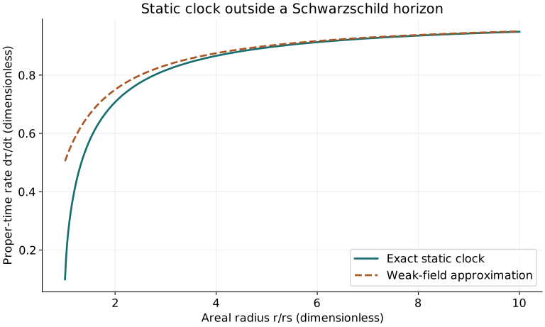
Example 07. Photon redshift from r=4rs to infinity

Definitions & inputs. A static emitter at re=4rs emits νe=600 THz; a static receiver is at infinity.

Review the governing derivation ↑

1. Use conservation of photon energy associated with the static time coordinate.

   $$\nu_o/\nu_e=\sqrt{1-r_s/r_e}=\sqrt{3/4}$$

2. The received frequency is lower.

   $$\nu_o=600\sqrt{3/4}=519.615\ {\rm THz}$$

3. Define the redshift as a wavelength increase, or inverse frequency ratio minus one.

   $$z=\nu_e/\nu_o-1=1/\sqrt{3/4}-1=0.154701$$

Interpretation. The frequency shift depends on the two observer worldlines.

• Tong — General Relativity: geometry, gravity, waves, and cosmology ↗

Example 08. Local radial proper distance near a black hole

Definitions & inputs. At r=2rs, take a small outward coordinate increment dr=1 m on a constant-t slice.

Review the governing derivation ↑

1. Hold time and angles fixed in the exterior metric.

   $$d\ell^2=\frac{dr^2}{1-r_s/r}$$

2. Substitute r=2rs.

   $$d\ell=dr/\sqrt{1-1/2}=\sqrt2\,dr$$

3. Areal-coordinate increments are not proper radial ruler distances.

   $$d\ell\simeq1.41421\ {\rm m}$$

Interpretation. For a finite interval, integrate dr/√(1−rs/r) instead of holding the factor constant.

• Tong — General Relativity: geometry, gravity, waves, and cosmology ↗

Example 09. Local radial escape speed at r=4rs

Definitions & inputs. A particle is launched outward at r=4rs; seek the speed relative to a local static observer needed to arrive at infinity with zero speed.

Review the governing derivation ↑

1. Relate conserved specific energy to locally measured Lorentz factor.

   $$e=\sqrt{1-r_s/r}\,\gamma_{\rm local},\quad e_{\rm escape}=1$$

2. Square and solve for the threshold speed.

   $$1=\sqrt{1-r_s/r}/\sqrt{1-v^2/c^2}\Rightarrow v^2/c^2=r_s/r$$

3. The algebra reproduces the familiar escape-speed form for this local measurement.

   $$r=4r_s\Rightarrow v=c/2=149896229\ {\rm m\,s^{-1}}$$

Interpretation. The local speed and coordinate speed are different quantities.

• Tong — General Relativity: geometry, gravity, waves, and cosmology ↗

Example 10. Circular orbit around a ten-solar-mass black hole

Definitions & inputs. M=10M⊙; choose r=10rg, where rg=GM/c².

Review the governing derivation ↑

1. The circular radial geodesic equation gives the coordinate angular frequency.

   $$\Omega^2=GM/r^3,\quad r=10GM/c^2$$

2. Substitute the chosen radius and convert angular frequency to cycles per second.

   $$\Omega=c^3/(10^{3/2}GM),\quad f_{\rm orb}=\Omega/(2\pi)$$

3. Evaluate with the specified mass.

   $$f_{\rm orb}=102.178\ {\rm Hz}$$

Interpretation. This is the orbital frequency, not twice that frequency used for dominant binary gravitational waves.

• Tong — General Relativity: geometry, gravity, waves, and cosmology ↗

Example 11. ISCO radius and ideal binding-energy efficiency

Definitions & inputs. M=10M⊙; rg=GM/c².

Review the governing derivation ↑

1. Apply circularity and marginal stability together.

   $$V_{\rm eff}^\prime=V_{\rm eff}^{\prime\prime}=0\Rightarrow r_{\rm ISCO}=6r_g$$

2. Evaluate the characteristic radius.

   $$r_{\rm ISCO}=6G(10M_\odot)/c^2=88.6002\ {\rm km}$$

3. Insert the circular-orbit angular momentum in the normalization relation.

   $$e(r)=\frac{1-2r_g/r}{\sqrt{1-3r_g/r}},\quad e_{\rm ISCO}=\sqrt{8/9}$$

4. This is the available orbital binding-energy fraction in the stated ideal model.

   $$\eta=1-e_{\rm ISCO}=0.057191=5.7191\%$$

Interpretation. Kerr spin changes both the ISCO and efficiency.

• Tong — General Relativity: geometry, gravity, waves, and cosmology ↗

Example 12. Mercury’s relativistic perihelion advance

Definitions & inputs. Use a=5.7909×10¹⁰ m, eccentricity eorb=0.20563, orbital period 87.969 days, M=M⊙.

Review the governing derivation ↑

1. Use the weak-field secular precession formula.

   $$\Delta\phi=6\pi GM/[ac^2(1-e_{\rm orb}^2)]$$

2. Insert orbital parameters.

   $$\Delta\phi=5.01882e-07\ {\rm rad/orbit}$$

3. Convert radians to arcseconds and multiply by orbits per Julian century.

   $$\Delta\phi_{\rm century}=\Delta\phi\frac{180(3600)}\pi\frac{36525}{87.969}=42.9821\ {\rm arcsec/century}$$

Interpretation. This is the relativistic contribution, not the total observed precession.

• Tong — General Relativity: geometry, gravity, waves, and cosmology ↗

Example 13. Light grazing the solar limb

Definitions & inputs. M=M⊙ and impact parameter b=R⊙=6.957×10⁸ m.

Review the governing derivation ↑

1. Use the two-asymptote null-geodesic deflection.

   $$\alpha=4GM/(bc^2)$$

2. Insert the grazing impact parameter.

   $$\alpha=8.49027e-06\ {\rm rad}$$

3. Convert the small angle to arcseconds.

   $$\alpha_{\rm arcsec}=\alpha(180/\pi)(3600)=1.75124$$

Interpretation. The leading GR bending is twice the result from a Newtonian corpuscular calculation.

• Tong — General Relativity: geometry, gravity, waves, and cosmology ↗

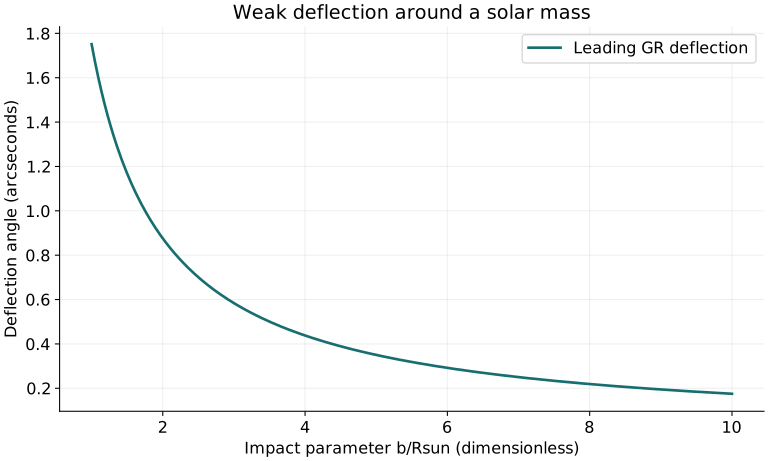
Example 14. Einstein ring of a stellar lens

Definitions & inputs. M=M⊙, DL=4 kpc, DS=8 kpc, DLS=4 kpc.

Review the governing derivation ↑

1. Combine α=4GM/(bc²), b≈DLθ, and the lens geometry.

   $$\beta=\theta-\frac{D_{LS}}{D_S}\frac{4GM}{c^2D_L\theta}$$

2. Alignment creates a ring; solve the lens equation for its angular radius.

   $$\beta=0\Rightarrow\theta_E=\sqrt{\frac{4GM D_{LS}}{c^2D_LD_S}}$$

3. Use 1 pc=3.08567758×10¹⁶ m and 1 mas=10⁻³ arcsec.

   $$\theta_E=1.00897\ {\rm mas}$$

Interpretation. This is a ring angle, not a physical radius at the source.

• Tong — General Relativity: geometry, gravity, waves, and cosmology ↗

Example 15. Round-trip solar Shapiro delay

Definitions & inputs. Take r1=1 AU, r2=1.5 AU and b=R⊙ near superior conjunction; M=M⊙.

Review the governing derivation ↑

1. A null path in the weak static metric receives both time and spatial-curvature contributions.

   $$dt\simeq(1-2\Phi/c^2)d\ell/c,\quad\Phi=-GM/r$$

2. Integrate along the unperturbed near-conjunction line; use distant-endpoint logarithmic limits.

   $$\Delta t_{\rm one}\simeq\frac{2GM}{c^3}\int\frac{dz}{\sqrt{b^2+z^2}}\simeq\frac{2GM}{c^3}\ln\frac{4r_1r_2}{b^2}$$

3. Double the one-way excess travel time for the idealized return path.

   $$\Delta t_{\rm round}\simeq\frac{4GM}{c^3}\ln\frac{4r_1r_2}{b^2}=246.939\ {\rm \mu s}$$

Interpretation. The delay is an excess over the corresponding flat-space travel-time model.

• Tong — General Relativity: geometry, gravity, waves, and cosmology ↗

Example 16. Radial tidal stretching near a stellar black hole

Definitions & inputs. M=10M⊙, r=10rs and radial separation ξ=2 m.

Review the governing derivation ↑

1. Geodesic deviation gives radial stretching; transverse separations are compressed.

   $$|\Delta a_r|=\frac{2GM}{r^3}\xi$$

2. Use the stated radius rather than confusing rs with rg.

   $$r=10r_s=20GM/c^2$$

3. Evaluate the acceleration difference across two metres.

   $$|\Delta a_r|=206084\ {\rm m\,s^{-2}}$$

Interpretation. Tidal acceleration depends strongly on radius and black-hole mass; it is not the acceleration of a static observer.

• Tong — General Relativity: geometry, gravity, waves, and cosmology ↗

Example 17. Convert gravitational-wave strain into arm displacement

Definitions & inputs. Plus-polarized amplitude h+=10⁻²¹; two orthogonal, aligned arms of length L=4000 m.

Review the governing derivation ↑

1. Expand the transverse-traceless spatial line element to first order.

   $$d\ell_x\simeq(1+h_+/2)dx,\quad d\ell_y\simeq(1-h_+/2)dy$$

2. Each arm has half the strain times baseline with opposite signs.

   $$\Delta L_x=h_+L/2=2\times10^{-18}\ {\rm m},\quad\Delta L_y=-2\times10^{-18}\ {\rm m}$$

3. The differential arm change contains the full factor hL.

   $$\Delta L_x-\Delta L_y=h_+L=4\times10^{-18}\ {\rm m}$$

Interpretation. Specify whether a quoted displacement refers to one arm or their difference.

• Tong — General Relativity: geometry, gravity, waves, and cosmology ↗

Example 18. Inspiral frequency growth at 100 Hz

Definitions & inputs. Chirp mass ℳ=1.21M⊙; gravitational-wave frequency f=100 Hz.

Review the governing derivation ↑

1. Use energy balance and Kepler’s relation derived above.

   $$\dot f=\frac{96}{5}\pi^{8/3}(G\mathcal M/c^3)^{5/3}f^{11/3}$$

2. Insert the chirp mass and measured wave frequency.

   $$\dot f=17.1572\ {\rm Hz\,s^{-1}}$$

3. Integrate the leading power law; the infinity upper limit defines a formal coalescence time.

   $$\dot f=Af^{11/3}\Rightarrow t_c-t=\int_f^\infty\frac{df^\prime}{A(f^\prime)^{11/3}}=\frac{3f}{8\dot f}$$

4. This is an approximate remaining inspiral time; the model is not valid all the way to infinite frequency.

   $$t_c-t\simeq2.18567\ {\rm s}$$

Interpretation. The steep f^(11/3) dependence produces the accelerating chirp.

• Tong — General Relativity: geometry, gravity, waves, and cosmology ↗

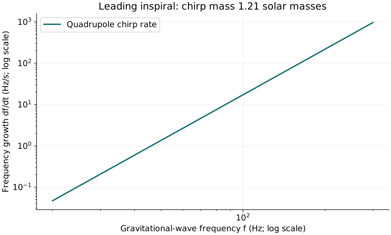
Example 19. Critical density for H0=70 km/s/Mpc

Definitions & inputs. H0=70 km s⁻¹ Mpc⁻¹; 1 Mpc=3.08567758×10²² m.

Review the governing derivation ↑

1. Convert the Hubble parameter to inverse seconds.

   $$H_0=70000/(3.08567758\times10^{22})=2.26855e-18\ {\rm s^{-1}}$$

2. Define the density scale associated with spatial flatness when all energy components are included consistently.

   $$\rho_{\rm crit}=3H_0^2/(8\pi G)$$

3. Square H0 and divide by the gravitational coupling.

   $$\rho_{\rm crit}=9.20387e-27\ {\rm kg\,m^{-3}}$$

Interpretation. Critical density is not automatically the baryon density or the density of a local material.

• Tong — General Relativity: geometry, gravity, waves, and cosmology ↗

Example 20. Age of an ideal flat matter-only universe

Definitions & inputs. Use H0=70 km s⁻¹ Mpc⁻¹ and normalize a(t0)=1.

Review the governing derivation ↑

1. Integrate conservation for pressureless matter.

   $$\dot\rho+3H\rho=0\Rightarrow\rho=\rho_0a^{-3}$$

2. Use the flat Friedmann equation and choose the expanding branch.

   $$H^2=H_0^2a^{-3}\Rightarrow\dot a=H_0a^{-1/2}$$

3. Set the big-bang origin at a=0,t=0 and integrate.

   $$\int_0^a a^{\prime1/2}da^\prime=H_0t\Rightarrow a=(3H_0t/2)^{2/3}$$

4. Apply a(t0)=1, converting seconds to Julian years.

   $$t_0=2/(3H_0)=9.31231\ {\rm Gyr}$$

Interpretation. Changing the matter/radiation/vacuum mixture changes the age–Hubble relation.

• Tong — General Relativity: geometry, gravity, waves, and cosmology ↗

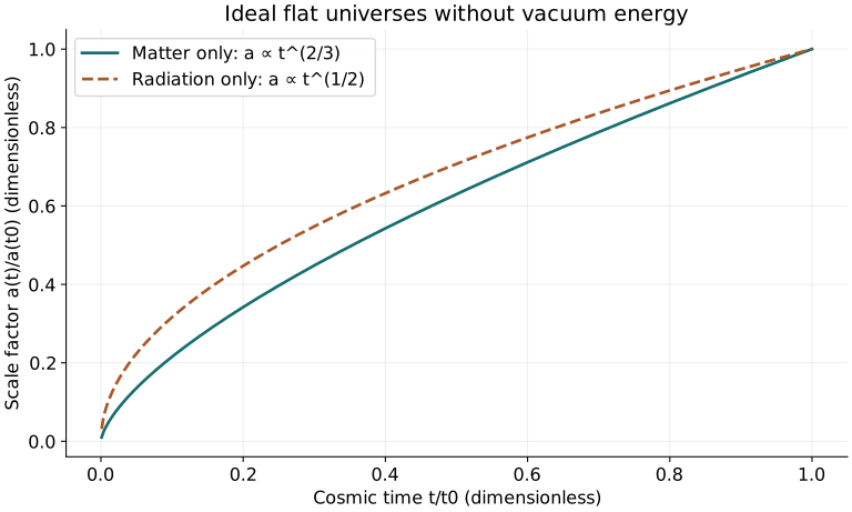
Connect gravity to atoms, solids, liquids, gases, and plasmas

Quantum mechanics determines atomic energy levels and material properties locally. Quantum field theory describes fields and many-body excitations; quantum fields on a prescribed curved spacetime do not by themselves constitute a complete quantum theory of gravity.

• Solids: an elastic stress tensor and an equation of state describe material response; ordinary terrestrial solids usually need only weak-field gravity.
• Liquids and gases: pressure, energy density, and flow enter the matter tensor; relativistic fluid equations use covariant conservation.
• Plasmas: combine fluid or kinetic matter with electromagnetic stress-energy for compact-star and accretion models. Strong fields, radiation, and composition may require additional microphysics.

Choose approximations independently: a plasma can be classical or quantum, weakly or strongly gravitating. Equations of state and transport laws close the matter equations; Einstein’s equation alone does not supply them.

Typical sensors and experimental connections

Interferometric displacement sensor · GNSS receiver · CCD image sensor

These are examples of instruments used to measure relevant observables, calibrate parameters, or test a physical system. They do not directly measure every abstract model quantity or prove a theory by themselves. Choose bandwidth, range, environment and uncertainty for the actual experiment.

Explore the dedicated Sensors site →

Mathematical tools and foundations

Metrics and distances · Tensors and change of basis

Use the stated mathematical conditions together with the physical assumptions. Explore the Mathematics atlas →