PHYSICS / ENGINEERING / COMPUTING
Plastic and viscoelastic deformation
Separate recoverable elasticity, permanent plastic strain and time-dependent response, then derive usable constitutive updates.
Matter pathway: atom → solid → liquid → gas → plasma. Quantum mechanics and quantum field theory provide foundations across the pathway; they are not additional phases. This is a connected modeling route, not a universal heating curve. Actual phases depend on pressure, composition, and kinetics.
1. Elastic–plastic split and yielding
Definitions & inputs. ε total strain,εe elastic strain,εp plastic strain,σy yield stress,H isotropic hardening modulus,α accumulated plastic strain.
Only the elastic strain supplies the linear elastic stress.
Define the elastic domain.
Plastic flow occurs on the yield surface; unloading can be elastic.
Interpretation. Residual strain after unloading distinguishes plasticity from reversible elasticity.
↑ Return to definitions and contents2. Return mapping
Definitions & inputs. σtrial elastic predictor,Δλ plastic multiplier,signs based on trial stress.
Hold plastic strain fixed for the trial step.
Impose the final yield condition to solve for the correction.
Update internal variables and recompute stress.
Interpretation. Multiaxial J2 plasticity uses von Mises stress and a tensor return map; a uniaxial formula is not that full algorithm.
↑ Return to definitions and contents3. Maxwell and Kelvin–Voigt rheology
Definitions & inputs. E spring stiffness,η dashpot viscosity,τ=η/E.
A Maxwell spring and dashpot in series share stress and add strains.
Under fixed strain the Maxwell model relaxes stress exponentially.
Parallel Kelvin–Voigt elements creep toward a finite strain under a stress step.
Interpretation. Maxwell creep is unbounded under sustained nonzero stress; Kelvin–Voigt has no instantaneous strain jump. Pick the model from measured behavior.
↑ Return to definitions and contents4. Generalized relaxation and dissipation
Definitions & inputs. E∞ long-time modulus,Ek positive modal moduli,τk relaxation times,ω angular frequency.
A spectrum of Maxwell branches adds relaxation time scales.
The in-phase storage modulus measures recoverable oscillatory response.
The loss modulus gives dissipated energy per unit volume per cycle.
Interpretation. Rate-dependent plastic flow requires additional yield and evolution laws. Time–temperature shifting is valid only over a characterized thermorheologically simple range.
↑ Return to definitions and contentsGraphical worked example
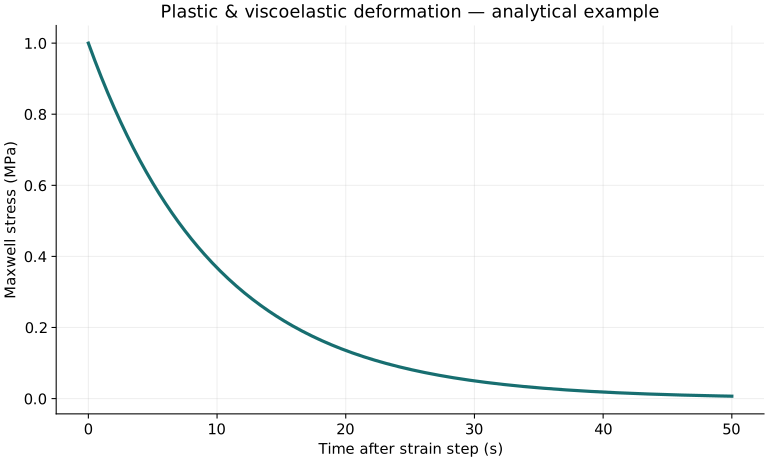
Twenty worked examples
Open a problem to see its defined inputs, assumptions, equation, numerical substitution, result, and interpretation. Values are illustrative analytical exercises.
Example 01. Elastic trial stress
Definitions & inputs. E200000MPa,ε.002,oldεp0.
Choose the governing model and isolate the requested quantity.
Insert the stated inputs in consistent units or the explicitly defined normalized units.
Evaluate the expression; the result uses the units shown.
Interpretation. Compare with the yield stress.
↑ Return to definitions and contentsExample 02. Yield function
Definitions & inputs. Trial400MPa,σy250MPa.
Choose the governing model and isolate the requested quantity.
Insert the stated inputs in consistent units or the explicitly defined normalized units.
Evaluate the expression; the result uses the units shown.
Interpretation. Positive trialf requires plastic correction.
↑ Return to definitions and contentsExample 03. Perfect-plastic increment
Definitions & inputs. E200000MPa,H0,trial400,yield250.
Choose the governing model and isolate the requested quantity.
Insert the stated inputs in consistent units or the explicitly defined normalized units.
Evaluate the expression; the result uses the units shown.
Interpretation. Monotone tensile step.
↑ Return to definitions and contentsExample 04. Corrected perfect-plastic stress
Definitions & inputs. Trial400MPa,E200000MPa,Δλ.00075.
Choose the governing model and isolate the requested quantity.
Insert the stated inputs in consistent units or the explicitly defined normalized units.
Evaluate the expression; the result uses the units shown.
Interpretation. Final stress lies on yield.
↑ Return to definitions and contentsExample 05. Hardening plastic increment
Definitions & inputs. Same but H10000MPa.
Choose the governing model and isolate the requested quantity.
Insert the stated inputs in consistent units or the explicitly defined normalized units.
Evaluate the expression; the result uses the units shown.
Interpretation. Isotropic linear hardening.
↑ Return to definitions and contentsExample 06. Hardening corrected stress
Definitions & inputs. σy0250MPa,H10000MPa,α150/210000.
Choose the governing model and isolate the requested quantity.
Insert the stated inputs in consistent units or the explicitly defined normalized units.
Evaluate the expression; the result uses the units shown.
Interpretation. Equals the corrected elastic stress.
↑ Return to definitions and contentsExample 07. Plastic tangent
Definitions & inputs. E200000MPa,H10000MPa.
Choose the governing model and isolate the requested quantity.
Insert the stated inputs in consistent units or the explicitly defined normalized units.
Evaluate the expression; the result uses the units shown.
Interpretation. Monotone plastic branch, not unloading slope.
↑ Return to definitions and contentsExample 08. Residual strain
Definitions & inputs. Total.002,stress250MPa,E200000MPa.
Choose the governing model and isolate the requested quantity.
Insert the stated inputs in consistent units or the explicitly defined normalized units.
Evaluate the expression; the result uses the units shown.
Interpretation. Fully unloading elastically retains this strain.
↑ Return to definitions and contentsExample 09. Von Mises pure shear
Definitions & inputs. τ100MPa.
Choose the governing model and isolate the requested quantity.
Insert the stated inputs in consistent units or the explicitly defined normalized units.
Evaluate the expression; the result uses the units shown.
Interpretation. J2 equivalent stress.
↑ Return to definitions and contentsExample 10. Pure shear yield
Definitions & inputs. Uniaxialσy250MPa.
Choose the governing model and isolate the requested quantity.
Insert the stated inputs in consistent units or the explicitly defined normalized units.
Evaluate the expression; the result uses the units shown.
Interpretation. Isotropic von Mises criterion.
↑ Return to definitions and contentsExample 11. Relaxation time
Definitions & inputs. η10⁹Pa·s,E10⁸Pa.
Choose the governing model and isolate the requested quantity.
Insert the stated inputs in consistent units or the explicitly defined normalized units.
Evaluate the expression; the result uses the units shown.
Interpretation. Maxwell or Kelvin characteristic time.
↑ Return to definitions and contentsExample 12. Maxwell initial stress
Definitions & inputs. E100MPa,stepε.01.
Choose the governing model and isolate the requested quantity.
Insert the stated inputs in consistent units or the explicitly defined normalized units.
Evaluate the expression; the result uses the units shown.
Interpretation. Immediately after ideal strain step.
↑ Return to definitions and contentsExample 13. Maxwell relaxed stress
Definitions & inputs. Initial1MPa,t10s,τ10s.
Choose the governing model and isolate the requested quantity.
Insert the stated inputs in consistent units or the explicitly defined normalized units.
Evaluate the expression; the result uses the units shown.
Interpretation. Maintained strain.
↑ Return to definitions and contentsExample 14. Stress half time
Definitions & inputs. τ10s.
Choose the governing model and isolate the requested quantity.
Insert the stated inputs in consistent units or the explicitly defined normalized units.
Evaluate the expression; the result uses the units shown.
Interpretation. Exponential relaxation.
↑ Return to definitions and contentsExample 15. Kelvin creep
Definitions & inputs. σ1MPa,E100MPa,t=τ.
Choose the governing model and isolate the requested quantity.
Insert the stated inputs in consistent units or the explicitly defined normalized units.
Evaluate the expression; the result uses the units shown.
Interpretation. Starts from zero strain.
↑ Return to definitions and contentsExample 16. Maxwell creep
Definitions & inputs. σ1MPa,E100MPa,η1000MPa·s,t20s.
Choose the governing model and isolate the requested quantity.
Insert the stated inputs in consistent units or the explicitly defined normalized units.
Evaluate the expression; the result uses the units shown.
Interpretation. Includes instant elastic and growing viscous strain.
↑ Return to definitions and contentsExample 17. Storage modulus
Definitions & inputs. Single Maxwell E10MPa,ωτ1,E∞0.
Choose the governing model and isolate the requested quantity.
Insert the stated inputs in consistent units or the explicitly defined normalized units.
Evaluate the expression; the result uses the units shown.
Interpretation. Oscillatory storage.
↑ Return to definitions and contentsExample 18. Loss modulus
Definitions & inputs. Same branch.
Choose the governing model and isolate the requested quantity.
Insert the stated inputs in consistent units or the explicitly defined normalized units.
Evaluate the expression; the result uses the units shown.
Interpretation. Loss peaks atωτ1 for this branch.
↑ Return to definitions and contentsExample 19. Cycle dissipation
Definitions & inputs. E″5MPa,strain amplitude.01.
Choose the governing model and isolate the requested quantity.
Insert the stated inputs in consistent units or the explicitly defined normalized units.
Evaluate the expression; the result uses the units shown.
Interpretation. Positive dissipation per cycle.
↑ Return to definitions and contentsExample 20. Long-time modulus
Definitions & inputs. Standard linear solidE∞2MPa,E1=8MPa,t≫τ.
Choose the governing model and isolate the requested quantity.
Insert the stated inputs in consistent units or the explicitly defined normalized units.
Evaluate the expression; the result uses the units shown.
Interpretation. Unlike a pure Maxwell fluid, this model retains stiffness.
↑ Return to definitions and contentsSymbols and units
Each derivation and problem defines its own symbols and inputs. Symbols may be reused with different meanings in other subjects. Keep units consistent, retain sufficient precision during calculation, and apply the stated validity limits.