Satellite design models

1. Mass and electrical budgets

Definitions & inputs. mi subsystem masses, Pi mode powers, di mode duty fractions, η conversion efficiency.

1. Aggregate mass and time-weighted load demand.

   $$M=\sum_i m_i,\quad P_{avg}=\sum_i d_iP_i$$

2. Size stored energy from load duration, usable depth of discharge, and discharge efficiency.

   $$E=P\Delta t,\quad E_{battery}=E_{load}/(\eta\,\mathrm{DOD})$$

3. Irradiance S, cell area A, incidence, and degradation set a first-order array output.

   $$P_{array}=S A\eta_{cell}\cos\theta\,d_{deg}$$

Worked example: Mode power and battery energy

Active mode 20 W for 25% of time, standby 4 W for 75%; eclipse load 12 W for 35 min, ηd=0.9 and DOD=0.8.

1. Weight each mutually exclusive mode by its duration fraction.

   $$P_{avg}=0.25(20)+0.75(4)=8\ \mathrm W$$

2. Calculate delivered eclipse energy using hours.

   $$E_e=12(35/60)=7\ \mathrm{Wh}$$

3. Apply discharge loss and usable depth of discharge; aging is omitted here.

   $$E_{nom}=7/(0.9\cdot0.8)=9.7222\ \mathrm{Wh}$$

Interpretation. Generation, eclipse energy, and peak power are separate constraints. Worked-example interpretation: This is a preliminary battery energy bound; section 6 closes the recharge and aging budget.

• NASA — Small Spacecraft Technology State of the Art ↗

2. Thermal balance

Definitions & inputs. α solar absorptivity, ε infrared emissivity, σSB Stefan–Boltzmann constant, Q internal heat.

1. Count absorbed external and internal heat.

   $$Q_{in}=\alpha S A_{proj}+Q_{internal}$$

2. Radiative rejection depends on radiating area and environment.

   $$Q_{rad}=\epsilon\sigma_{SB}A(T^4-T_{sink}^4)$$

3. Thermal mass governs transients rather than the steady equilibrium alone.

   $$mc_p\,dT/dt=Q_{in}-Q_{out}$$

Worked example: Size an ideal radiator

Qinternal=20 W, no absorbed sunlight or Earth flux, ε=0.8, T=300 K and Ts≈0 K.

1. Specify the deliberately isolated heat-input case.

   $$Q_{in}=20+0=20\ \mathrm W$$

2. Calculate radiated flux per unit area.

   $$\epsilon\sigma T^4=367.440\ \mathrm{W/m^2}$$

3. Divide required rejection by radiative flux.

   $$A=20/367.440=0.0544306\ \mathrm{m^2}$$

Interpretation. Do not confuse illuminated projected area with total radiating area. Worked-example interpretation: Absorbed external heat or obstructed view increases required area; this is not a complete orbital hot case.

• NASA — Small Spacecraft Technology State of the Art ↗

3. Communications and data return

Definitions & inputs. Pt transmit power, Gt,Gr antenna gains, λ wavelength, R range, Rb bit rate, Ts system noise temperature.

1. Friis combines spherical spreading with effective receive aperture.

   $$P_r=P_tG_tG_r(\lambda/4\pi R)^2$$

2. Convert spreading loss into decibels.

   $$L_{fs}=20\log_{10}(4\pi R/\lambda)$$

3. Received energy per bit is compared with noise spectral density; implementation and coding set required margin.

   $$E_b/N_0=P_r/(k_BT_sR_b)$$

Worked example: Range loss and information energy

Frequency=2 GHz, R=1000 km; separately assume received carrier power Pr=10⁻¹³ W, Tsys=500 K and Rb=100000 bit/s.

1. Convert frequency to wavelength.

   $$\lambda=c/f=0.149896\ \mathrm m$$

2. Compute the geometric spreading loss; received power is a separate given input in this example.

   $$L_{fs}=20\log_{10}(4\pi R/\lambda)=158.468\ \mathrm{dB}$$

3. First calculate the dimensionless linear ratio; use ten times its logarithm for decibels.

   $$E_b/N_0=10^{-13}/[k_B(500)(10^5)]=144.859\simeq21.610\ \mathrm{dB}$$

Interpretation. A positive free-space budget alone does not guarantee coverage or availability. Worked-example interpretation: Section 8 connects transmitted power and antenna gains to the received-power input used here.

• NASA — Small Spacecraft Technology State of the Art ↗

4. Pointing and payload geometry

Definitions & inputs. τ torque, J inertia, ω angular speed, θ pointing error, h altitude, f focal length, p pixel pitch.

1. Torque changes angular rate and stored wheel momentum.

   $$J\dot\omega=\tau,\quad\Delta H=\tau\Delta t$$

2. Pixel angular width maps to ground sampling distance.

   $$\mathrm{GSD}\simeq hp/f$$

3. Pointing error translates to a ground displacement near nadir.

   $$\Delta x\simeq h\theta$$

Worked example: Pointing displacement and pixel footprint

H=500 km, pointing error=10 μrad, pixel pitch=5 μm and focal length=0.5 m.

1. Divide pitch by focal length.

   $$\delta\theta_{pix}=5\times10^{-6}/0.5=10^{-5}\ \mathrm{rad}$$

2. Map angular sampling to the ground.

   $$\mathrm{GSD}=500000(10^{-5})=5\ \mathrm m$$

3. A 10 μrad pointing offset moves the footprint by one pixel in this geometry.

   $$\Delta x=500000(10\times10^{-6})=5\ \mathrm m$$

Interpretation. Sampling distance is not the same as optical resolution or geolocation accuracy. Worked-example interpretation: A constant offset affects location; fluctuating pointing during exposure also blurs the image.

• NASA — Small Spacecraft Technology State of the Art ↗

5. Derive eclipse duration from orbit geometry

Definitions & inputs. r is geocentric orbit radius, RE Earth radius, β Sun elevation above the orbit plane, ψ eclipse half-angle, n mean motion, To orbital period.

1. Equate radial gravitational acceleration to centripetal acceleration. A full revolution then takes 2π divided by angular rate.

   $$n=\sqrt{\mu/r^3},\qquad T_o=2\pi/n$$

2. At shadow entry, resolve the position into components parallel and perpendicular to the Sun direction, measuring ψ from anti-solar conjunction.

   $$d_\perp^2=r^2(1-\cos^2\beta\cos^2\psi)$$

3. Set the perpendicular distance equal to Earth radius. The spacecraft must also be behind Earth to be in eclipse.

   $$\cos\psi_e=\frac{\sqrt{1-(R_E/r)^2}}{\cos\beta}$$

4. A real shadow crossing exists only below the critical beta angle; otherwise eclipse duration is zero. At equality the shadow is tangent.

   $$|\beta|<\arcsin(R_E/r),\qquad t_e=2\psi_e/n$$

5. At zero beta, a right triangle gives the eclipse half-angle directly. This is the longest cylindrical eclipse for this circular orbit.

   $$\beta=0:\quad t_e=\frac{T_o}{\pi}\arcsin(R_E/r)$$

Worked example: 500 km circular orbit at zero beta

Use RE=6371 km, r=6871 km and μ=398600.4418 km³/s²; angles are radians inside trigonometric functions.

1. Compute the full orbital period.

   $$T_o=2\pi\sqrt{6871^3/398600.4418}=5668.14\ \mathrm{s}$$

2. Use radius rather than altitude in the shadow triangle.

   $$\psi_e=\arcsin(6371/6871)\simeq1.187\ \mathrm{rad}$$

3. Multiply the shadow fraction by the period.

   $$t_e\simeq2141.523\ \mathrm{s}\simeq35.692\ \mathrm{min}$$

Interpretation. Eclipse is a geometry constraint that drives both battery capacity and cold-case thermal design. Worked-example interpretation: An actual mission must evaluate beta angle through the season, not size from sunlight duty alone.

• NASA — Small Spacecraft Technology State of the Art ↗

6. Close the sunlight, eclipse and end-of-life power budget

Definitions & inputs. Ps and Pe are bus loads during sunlight and eclipse; ts and te are their durations; ηd discharge efficiency, ηc charge efficiency, D usable depth of discharge, fcap remaining battery capacity fraction.

1. Integrate the eclipse load. The battery must release more stored energy than reaches the bus when discharge efficiency is below unity.

   $$E_e=P_et_e,\qquad E_{\mathrm{stored,used}}=E_e/\eta_d$$

2. Only the specified depth of discharge and remaining capacity are usable. This is an energy bound, separate from peak-current and voltage constraints.

   $$E_{\mathrm{nom}}\geq\frac{P_et_e}{\eta_d D f_{cap}}$$

3. Periodic steady operation requires the array to serve the sunlit load and restore the stored energy removed in eclipse.

   $$P_{\mathrm{array,bus}}t_s=P_st_s+\frac{P_et_e}{\eta_c\eta_d}$$

4. Divide by sunlit time. Sizing the array to orbit-average load without charging losses understates the requirement.

   $$P_{\mathrm{array,bus}}\geq P_s+\frac{P_et_e}{\eta_c\eta_dt_s}$$

5. Convert bus power to cell area using end-of-life degradation, conversion loss, and sunlit average projected orientation. Shadowing is an additional factor if present.

   $$A\geq\frac{P_{\mathrm{array,bus}}}{S\eta_{cell}\eta_{bus}f_{deg}\langle\max(0,\cos\theta)\rangle_s}$$

Worked example: One illustrative 95-minute orbit

Ps=20 W, Pe=12 W, ts=60 min, te=35 min, ηc=ηd=0.9, D=0.6, fcap=0.8; S=1361 W/m², cell efficiency 0.30, bus efficiency 0.90, degradation 0.80, mean cosine 0.75.

1. Convert minutes to hours for the battery calculation.

   $$E_{nom}\geq\frac{12(35/60)}{0.9(0.6)(0.8)}=16.204\ \mathrm{Wh}$$

2. The array must provide 8.642 W above the sunlit load for charging.

   $$P_{array,bus}\geq20+\frac{12(35)}{0.9^2(60)}=28.642\ \mathrm W$$

3. Use cell area; panel substrate, gaps and mechanical margins add to physical panel area.

   $$A\geq28.642/[1361(0.30)(0.90)(0.80)(0.75)]=0.12990\ \mathrm{m^2}$$

Interpretation. A feasible energy balance still needs verification of peak loads, battery charge rate, cold temperature and bus voltage. Worked-example interpretation: The larger energy-storage allowance follows from aging and depth-of-discharge limits, not an increase in delivered eclipse energy.

• NASA — Small Spacecraft Technology: Power ↗

7. Derive a thermal network and its response time

Definitions & inputs. Ci=mi cpi is node heat capacity in J/K, Gij conductance in W/K, Qi heat input, Ai radiator area, εi emissivity, Ts radiative sink temperature.

1. Fourier conduction through a uniform link gives a heat flow proportional to temperature difference. Contact resistance can dominate the bulk link.

   $$Q_{ij}=G_{ij}(T_j-T_i),\qquad G_{ij}=kA_c/\ell$$

2. Apply conservation of energy to each node. Equal and opposite conduction terms cancel when summing the whole spacecraft.

   $$C_i\dot T_i=Q_i+\sum_jG_{ij}(T_j-T_i)-\epsilon_i\sigma A_i(T_i^4-T_s^4)$$

3. A one-node equilibrium has zero energy accumulation. Solar, albedo, Earth infrared and internal dissipation must be included in Q0 at the relevant geometry.

   $$Q_0=\epsilon\sigma A(T_0^4-T_s^4)$$

4. Taylor-expand radiative loss about equilibrium and subtract the equilibrium balance. Discard terms quadratic and higher in the temperature perturbation.

   $$T=T_0+\delta T:\quad C\delta\dot T+4\epsilon\sigma AT_0^3\delta T=\delta Q$$

5. For a step heat input and initially zero perturbation, the linearized temperature approaches its new value exponentially.

   $$\tau_T=\frac{C}{4\epsilon\sigma AT_0^3},\quad\delta T(t)=\frac{\delta Q}{4\epsilon\sigma AT_0^3}(1-e^{-t/\tau_T})$$

Worked example: A small radiator near 300 K

C=900 J/K, ε=0.8, A=0.10 m², σ=5.670374419×10⁻⁸ W/m²/K⁴, Ts≈0 K; apply an extra 1 W.

1. Find the equilibrium heat load for this temperature.

   $$Q_0=0.8\sigma(0.10)(300)^4=36.744\ \mathrm W$$

2. Differentiate the radiation law, then divide heat capacity by the slope.

   $$G_{rad}=4\epsilon\sigma AT_0^3=0.48992\ \mathrm{W/K},\quad\tau_T=1837.03\ \mathrm s$$

3. At one time constant, the linear model reaches 63.2 percent of its 2.041 K eventual rise.

   $$\delta T(\tau_T)=\frac{1}{0.48992}(1-e^{-1})=1.2903\ \mathrm K$$

Interpretation. Large hot/cold excursions require the nonlinear differential equations; a local time constant is not a substitute for an orbit thermal simulation. Worked-example interpretation: The small predicted rise is consistent with linearizing around 300 K.

• NASA — Small Spacecraft Technology: Thermal Control ↗

8. Derive a radio link from flux to usable data

Definitions & inputs. Pt transmitted RF power, Gt and Gr linear gains, R range, λ wavelength, Ae receiver effective area, L≥1 aggregate linear loss, kB Boltzmann constant, Tsys noise temperature, Rb bit rate.

1. Spread transmitted power over a sphere and convert receiving gain to effective collecting area.

   $$F=\frac{P_tG_t}{4\pi R^2},\qquad A_e=\frac{G_r\lambda^2}{4\pi}$$

2. Multiply flux by collecting area; propagation, pointing and implementation losses must be allocated consistently.

   $$P_r=FA_e/L=\frac{P_tG_tG_r}{L}\left(\frac{\lambda}{4\pi R}\right)^2$$

3. Noise spectral density has units W/Hz; dividing carrier-to-noise-density ratio by bits per second yields energy per bit relative to noise density.

   $$N_0=k_BT_{sys},\quad C/N_0=P_r/(k_BT_{sys}),\quad E_b/N_0=\frac{P_r}{k_BT_{sys}R_b}$$

4. Taking ten times the base-ten logarithm turns products into sums; 228.599 is minus ten times the logarithm of kB in SI units.

   $$(C/N_0)_{dBHz}=P_{r,dBW}+228.599-10\log_{10}T_{sys}$$

5. Subtract the required modem threshold after all separately budgeted losses. Margin is not data volume; contact time determines the latter.

   $$M=(C/N_0)_{dBHz}-10\log_{10}R_b-(E_b/N_0)_{req,dB}$$

Worked example: A hypothetical 1 Mbit/s downlink

Pt=2 W, Gt=3 dBi, Gr=30 dBi, frequency=2 GHz, R=1000 km, aggregate loss=3 dB, Tsys=500 K; assumed required Eb/N0=6 dB.

1. Use c=299792458 m/s and range in metres.

   $$L_{fs}=20\log_{10}(4\pi Rf/c)=158.468\ \mathrm{dB}$$

2. Convert 2 W to 3.0103 dBW before adding logarithmic gains.

   $$P_r=3.0103+3+30-158.4684-3=-125.4581\ \mathrm{dBW}$$

3. Subtract 60 dB for one million bits per second, then the assumed 6 dB threshold.

   $$E_b/N_0=16.151\ \mathrm{dB},\qquad M=10.151\ \mathrm{dB}$$

Interpretation. The communications chapter provides technology context; the derivation here is an ideal analytical link budget, not measured hardware performance. Worked-example interpretation: Doubling range loses 6.02 dB. The threshold is an exercise input; real coding, weather and antenna patterns set the actual requirement.

• NASA — Small Spacecraft Technology: Communications ↗

9. Rigid-body attitude, wheel momentum and controlled slews

Definitions & inputs. J is the body inertia tensor, ω body angular velocity, hw wheel momentum expressed in body axes, τext external torque; θ slew angle and ts slew duration.

1. Total angular momentum includes both the spacecraft body and spinning wheels.

   $$\mathbf H=J\boldsymbol\omega+\mathbf h_w$$

2. The inertial time derivative of a vector equals its body derivative plus ω cross the vector. Internal wheel torque redistributes momentum; it does not remove total momentum.

   $$J\dot{\boldsymbol\omega}+\boldsymbol\omega\times(J\boldsymbol\omega+\mathbf h_w)=\boldsymbol\tau_{ext}-\dot{\mathbf h}_w$$

3. During a symmetric triangular rate profile, total angle is the area under angular rate versus time.

   $$\theta=2\left(\tfrac12\alpha(t_s/2)^2\right)=\alpha t_s^2/4$$

4. Solve for commanded acceleration, torque and midpoint angular rate. Wheel capability and structural settling may impose slower motion.

   $$\alpha=4\theta/t_s^2,\quad\tau=J\alpha,\quad\omega_{max}=2\theta/t_s$$

5. A persistent disturbance fills wheel storage. A magnetic torquer can unload momentum only perpendicular to the local field; instantaneous three-axis torque is unavailable.

   $$t_{sat}\simeq H_{available}/|\tau_{bias}|,\qquad\boldsymbol\tau_{mag}=\mathbf m\times\mathbf B$$

Worked example: A 10-degree rest-to-rest slew

J=0.20 kg m², ts=20 s, θ=10π/180 rad. For a separate unloading estimate use available momentum 0.02 N m s and bias torque 10⁻⁵ N m.

1. Convert degrees to radians before calculating angular acceleration.

   $$\alpha=4(10\pi/180)/20^2=0.00174533\ \mathrm{rad/s^2}$$

2. The wheel must supply both sufficient torque and sufficient speed/momentum headroom.

   $$\tau=0.000349066\ \mathrm{N\,m},\quad\omega_{max}=0.0174533\ \mathrm{rad/s}$$

3. Estimate time to saturation under a constant unopposed bias.

   $$t_{sat}=0.02/10^{-5}=2000\ \mathrm s$$

Interpretation. Pointing accuracy also depends on attitude knowledge, sensor bias, jitter and controller bandwidth, which a torque-only calculation omits. Worked-example interpretation: A wheel that can execute the slew may still saturate within about 33 minutes of sustained bias.

• NASA — Small Spacecraft Technology: Guidance, Navigation and Control ↗

10. Connect pixel sampling, diffraction and image motion

Definitions & inputs. H altitude, p detector pitch, f focal length, D aperture diameter, λ wavelength, σθ pointing jitter, vg image ground speed, texp exposure time.

1. Similar triangles map a detector pixel to an angular interval and then a projected ground interval.

   $$\delta\theta_{pix}\simeq p/f,\qquad\mathrm{GSD}\simeq Hp/f$$

2. Diffraction spreads light from a point source. Smaller pixels do not remove this optical limit.

   $$\theta_{Rayleigh}=1.22\lambda/D,\quad\ell_{Rayleigh}\simeq1.22H\lambda/D$$

3. Map small pointing jitter to ground displacement and integrate uncompensated image motion during an exposure.

   $$\sigma_x=H\sigma_\theta,\qquad\ell_{smear}=v_gt_{exp}$$

4. A uniform line smear convolves the image with a box kernel; its Fourier transform is a sinc. q is ground spatial frequency in cycles per metre.

   $$\mathrm{MTF}_{smear}(q)=\left|\frac{\sin(\pi q\ell_{smear})}{\pi q\ell_{smear}}\right|$$

5. Independent shift-invariant blur kernels convolve in space and multiply in spatial frequency. Atmosphere and processing can add further factors.

   $$\mathrm{MTF}_{total}=\mathrm{MTF}_{optics}\,\mathrm{MTF}_{pixel}\,\mathrm{MTF}_{jitter}\,\mathrm{MTF}_{smear}$$

Worked example: A 500 km imaging payload

H=500000 m, p=5 μm, f=0.50 m, D=0.10 m, λ=550 nm, σθ=2 μrad, vg=7500 m/s, exposure=0.5 ms.

1. Compute the pixel footprint.

   $$\mathrm{GSD}=500000(5\times10^{-6})/0.50=5.0\ \mathrm m$$

2. Compare the diffraction criterion to the sample spacing without calling either the final resolution.

   $$\ell_{Rayleigh}=1.22(500000)(550\times10^{-9})/0.10=3.355\ \mathrm m$$

3. Even a sub-millisecond exposure can produce appreciable uncompensated smear.

   $$\sigma_x=1.0\ \mathrm m,\quad\ell_{smear}=7500(0.0005)=3.75\ \mathrm m$$

Interpretation. Ground sampling distance is a sampling scale; resolved detail and geolocation require separate optical, motion and navigation budgets. Worked-example interpretation: The 3.75 m smear is 0.75 pixel; time-delay integration or image-motion compensation changes this budget.

• NASA — Small Spacecraft Technology State of the Art ↗

11. Derive propellant mass and expose mass feedback

Definitions & inputs. m is instantaneous spacecraft mass, ve=Isp g0 exhaust speed, md final dry mass including tanks and hardware, mp usable propellant, Δv ideal velocity increment.

1. Conserve momentum over a short ejection interval. Spacecraft mass decreases, so dm is negative and a positive exhaust speed produces a positive velocity increment.

   $$m\,dv=-v_e\,dm$$

2. Integrate the changing mass rather than assuming constant acceleration or constant spacecraft mass.

   $$\Delta v=-v_e\int_{m_0}^{m_f}\frac{dm}{m}=v_e\ln(m_0/m_f)$$

3. Set final mass equal to dry mass for this usable-propellant idealization, then isolate propellant.

   $$m_p=m_d[\exp(\Delta v/v_e)-1]$$

4. If tank mass scales with propellant, substitute the dry-mass relation and solve the algebraic feedback loop. A positive finite solution requires kt q below one.

   $$m_d=m_{base}+k_tm_p\quad\Longrightarrow\quad m_p=\frac{m_{base}q}{1-k_tq},\quad q=e^{\Delta v/v_e}-1$$

5. For fixed dry mass, differentiate to show why additional velocity margin costs progressively more propellant.

   $$\frac{\partial m_p}{\partial\Delta v}=\frac{m_d}{v_e}e^{\Delta v/v_e}$$

Worked example: Station-keeping allocation for a small spacecraft

md=20 kg, Δv=100 m/s, Isp=220 s and g0=9.80665 m/s²; dry mass is fixed for this calculation.

1. Convert specific impulse to effective exhaust velocity.

   $$v_e=220(9.80665)=2157.463\ \mathrm{m/s}$$

2. Calculate the required propellant-to-dry-mass ratio.

   $$q=e^{100/2157.463}-1=0.0474417$$

3. Add this to dry mass to obtain initial wet mass, before residuals and operational reserves.

   $$m_p=20q=0.948834\ \mathrm{kg}$$

Interpretation. Trajectory Δv, thruster performance and dry-mass estimates must converge together; percentage mass reserves do not replace a maneuver inventory. Worked-example interpretation: A 100 m/s requirement is not a universal station-keeping value; it is an illustrative input.

• NASA — Small Spacecraft Technology State of the Art ↗

12. Launch loads, stiffness and structural resonance

Definitions & inputs. m effective modal mass, k modal stiffness, c damping, x relative displacement, ay base acceleration, E Young modulus, I area second moment, L beam length.

1. Write force balance in the accelerating support frame. A static acceleration is only the zero-frequency limit of the launch excitation.

   $$m\ddot x+c\dot x+kx=-ma_y(t)$$

2. The homogeneous characteristic equation defines natural frequency and damping ratio.

   $$\omega_n=\sqrt{k/m},\quad f_n=\omega_n/(2\pi),\quad\zeta=c/(2\sqrt{km})$$

3. For a tip-loaded cantilever, Euler–Bernoulli bending gives equivalent tip stiffness. Different attachments require a different stiffness model.

   $$k=3EI/L^3,\qquad x_{static}=ma_y/k$$

4. Substitute sinusoidal excitation into the differential equation and take the magnitude of the complex compliance.

   $$\frac{|x|}{ma_0/k}=\frac{1}{\sqrt{(1-r_f^2)^2+(2\zeta r_f)^2}},\quad r_f=\omega/\omega_n$$

5. At the undamped natural frequency, a low-damping structure can amplify the static displacement substantially; the exact peak shifts slightly when damping is nonzero.

   $$r_f=1:\quad\frac{|x|}{ma_0/k}=\frac{1}{2\zeta}$$

Worked example: An illustrative instrument mounting mode

m=2 kg, k=200000 N/m, ζ=0.05; use 6g as a static equivalent load and g0=9.80665 m/s².

1. Calculate the frequency of the single-mode approximation.

   $$f_n=\sqrt{200000/2}/(2\pi)=50.329\ \mathrm{Hz}$$

2. The static displacement is about 0.588 mm.

   $$x_{static}=2(6)(9.80665)/200000=0.000588399\ \mathrm m$$

3. A harmonic load at this natural frequency would produce ten times its own static-response amplitude in this linear model.

   $$1/(2\zeta)=10$$

Interpretation. Strength, buckling, fatigue and modal separation are distinct checks; passing one does not establish the others. Worked-example interpretation: The 6g static example is not a prescribed sinusoidal test; use the actual excitation spectrum to compute dynamic response.

• NASA — Small Spacecraft Technology State of the Art ↗

13. Separate reliability, redundancy and radiation events

Definitions & inputs. λf constant failure rate, R reliability over duration t, σSEE event cross-section, Φ particle flux, ν expected count; component failures and recoverable upsets are distinct events.

1. Survival over the next interval requires survival so far and no new failure. Taking the small-time limit produces the hazard differential equation.

   $$R(t+dt)=R(t)(1-\lambda_fdt)\quad\Longrightarrow\quad\dot R=-\lambda_f R$$

2. Solve the survival equation; multiply independent essential-component reliabilities for series operation and independent failure probabilities for parallel redundancy.

   $$R(t)=e^{-\lambda_ft},\quad R_{series}=\prod_iR_i,\quad R_{parallel}=1-\prod_i(1-R_i)$$

3. Fold measured device susceptibility with the radiation spectrum. A Poisson model converts mean event count into probability of at least one event.

   $$\nu=t\int\sigma_{SEE}(E)\Phi(E)\,dE,\quad P(N\geq1)=1-e^{-\nu}$$

4. A spectrum-averaged effective cross-section reduces the integral to a scalar estimate when the averaging matches the environment.

   $$\nu=\sigma_{eff}\Phi_{tot}t$$

5. If a separate common-cause event with probability qc defeats both channels, independent redundancy gains are reduced. Switching and recovery coverage require additional factors.

   $$R_{parallel,common}=(1-q_c)[1-(1-R)^2]$$

Worked example: Redundancy and a separate upset estimate

Two independent channels each R=0.95 over the mission; independent common-cause probability qc=0.02. Separately, σeff=10⁻⁶ cm²/device, Φtot=100 cm⁻²s⁻¹ and t=10000 s.

1. Calculate the ideal redundant-channel reliability.

   $$R_{parallel}=1-0.05^2=0.9975$$

2. Include the explicitly separate common-cause event.

   $$R_{parallel,common}=0.98(0.9975)=0.97755$$

3. The event probability is about 63.2 percent even though the mean is just one upset.

   $$\nu=10^{-6}(100)(10000)=1,\quad P(N\geq1)=1-e^{-1}=0.632121$$

Interpretation. Total ionizing dose, displacement damage, latchup and transient upsets require different response models; an upset count is not automatically a catastrophic-failure probability. Worked-example interpretation: Error correction and recovery can make an upset survivable; do not substitute the upset probability for the subsystem reliability.

• NASA — Small Spacecraft Technology State of the Art ↗

14. Close the payload-to-ground data budget

Definitions & inputs. Rg raw payload bit rate, d duty fraction, ccomp raw-to-compressed size ratio, To orbit duration, Rnet usable downlink information rate, tc contact time, B stored backlog.

1. Multiply pixels per frame by bits per pixel and frames per second; include all bands and metadata when specifying a real payload.

   $$R_{raw}=N_{pix}\,b\,f_{frame}$$

2. Integrate acquisition time and apply a stated compression factor. Lossy compression may change the science or image-quality requirement.

   $$D_{gen}=R_{raw}dT_o/c_{comp}$$

3. Use a period-end queue balance when the generated data are available for the scheduled downlink; actual event timing is needed to determine peak storage.

   $$D_{down}=R_{net}t_c,\quad B_{k+1}=\max(0,B_k+D_{gen,k}-D_{down,k})$$

4. Long-term stability requires mean service to cover mean generation. Strict surplus provides room to recover from missed contacts.

   $$\langle D_{down}\rangle\geq\langle D_{gen}\rangle$$

5. Propagate the time history with service limited by queue availability. Capacity depends on the worst accumulated backlog, not only an average balance.

   $$B_{peak}=\max_t\left[B(0)+\int_0^t(R_{gen}-R_{served})\,dt\right]$$

Worked example: Data return over a 95-minute orbit

A compressed payload generates 8 Mbit/s for 10 min each orbit. A usable 20 Mbit/s downlink is available for 5 min after acquisition. Decimal units are used.

1. Ten minutes of data correspond to 600 MB before file-system and protection overhead.

   $$D_{gen}=8\times10^6(600)=4.8\times10^9\ \mathrm{bit}$$

2. The nominal contact can remove 750 MB, leaving 150 MB of spare service per orbit.

   $$D_{down}=20\times10^6(300)=6.0\times10^9\ \mathrm{bit}$$

3. One missed pass leaves 600 MB; after the next acquisition peak backlog is 1200 MB. Four successful orbits are needed to remove the extra 600 MB using spare capacity.

   $$B_{missed}=2(600)=1200\ \mathrm{MB},\quad N_{recovery}=600/(750-600)=4$$

Interpretation. A positive link margin does not ensure enough contact time, and sufficient average contact time does not ensure enough buffer capacity. Worked-example interpretation: This schedule needs at least 1.2 GB for the illustrated single missed pass, before storage margin and overhead.

• NASA — Small Spacecraft Technology: Communications ↗

Graphical worked example

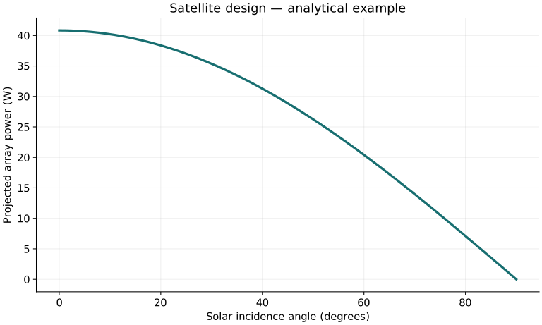
Twenty worked examples

Open a problem to see its defined inputs, assumptions, equation, numerical substitution, result, and interpretation. Values are illustrative analytical exercises.

Connect this subject to other models

• Astrodynamics and orbital mechanics
• Optics models
• Reliability calculation models
• Survivability under environmental stresses and faults
• Sensor types, measurement models and calibration
• Spaceflight trajectory calculation
• Heat transfer models
• Communication systems and signal processing
• Control theory models

Return to the subject library · Numerical solution techniques

Typical sensors and experimental connections

Star tracker · MEMS vibrating gyroscope · Thermistor

These are examples of instruments used to measure relevant observables, calibrate parameters, or test a physical system. They do not directly measure every abstract model quantity or prove a theory by themselves. Choose bandwidth, range, environment and uncertainty for the actual experiment.

Explore the dedicated Sensors site →

Mathematical tools and foundations

Derivatives and chain rule · Linear systems and elimination · Monte Carlo estimation

Use the stated mathematical conditions together with the physical assumptions. Explore the Mathematics atlas →