PHYSICS / ENGINEERING / COMPUTING
Communication systems and signal processing
Follow sampling, linear filters, noise, information rate, modulation, and link margins through twenty worked calculations.
Matter pathway: atom → solid → liquid → gas → plasma. Quantum mechanics and quantum field theory provide foundations across the pathway; they are not additional phases. This is a connected modeling route, not a universal heating curve. Actual phases depend on pressure, composition, and kinetics.
1. Sampling and spectra
Definitions & inputs. fs sample frequency, B highest frequency of a real baseband signal, N sample count.
Sampling replicates spectra; separation prevents overlap for generic baseband signals.
A record of duration T sets DFT-bin spacing.
Choose integer m to fold a real sinusoid into the Nyquist interval.
Interpretation. DFT bin spacing is not automatically the ability to resolve nearby tones; windowing matters.
↑ Return to definitions and contents2. Linear filtering
Definitions & inputs. x[n] input, h[n] impulse response, y[n] output, H frequency response.
Sum the shifted impulse responses weighted by input samples.
Transform convolution into multiplication in frequency.
A two-sample average has cosine magnitude and a half-sample linear phase delay.
Interpretation. Boundary handling and filter transient state must be defined for finite records.
↑ Return to definitions and contents3. Noise and capacity
Definitions & inputs. k Boltzmann constant, T noise temperature, B equivalent noise bandwidth, S signal power, N noise power.
Integrate the flat available noise power density across bandwidth.
Shannon’s AWGN limit bounds reliable rate with ideal coding and arbitrarily long blocks.
Divide signal power by bit rate and noise power by bandwidth consistently.
Interpretation. Real coding, latency, interference and nonwhite noise change achievable performance.
↑ Return to definitions and contents4. Digital modulation
Definitions & inputs. M constellation size, Rs symbols/s, Rb bits/s, α roll-off; γb=Eb/N0.
Count bits per symbol and spectral support around the carrier.
Project AWGN onto the coherent decision axis and integrate the error tail.
Code rate rc reduces payload before additional framing overhead.
Interpretation. Synchronization, fading, nonlinearities and detection method must match the BER model.
↑ Return to definitions and contentsGraphical worked example
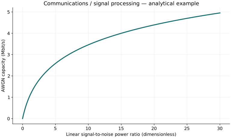
Twenty worked examples
Open a problem to see its defined inputs, assumptions, equation, numerical substitution, result, and interpretation. Values are illustrative analytical exercises.
Example 01. Nyquist threshold
Definitions & inputs. Real baseband content up to 20 kHz.
Choose the governing model and isolate the requested quantity.
Insert the stated inputs in consistent units or the explicitly defined normalized units.
Evaluate the expression; the result uses the units shown.
Interpretation. Practical sampling exceeds this threshold to allow filter transition bands.
↑ Return to definitions and contentsExample 02. Sample interval
Definitions & inputs. fs=48000 samples/s.
Choose the governing model and isolate the requested quantity.
Insert the stated inputs in consistent units or the explicitly defined normalized units.
Evaluate the expression; the result uses the units shown.
Interpretation. This is the ideal uniform sampling period.
↑ Return to definitions and contentsExample 03. Aliased sinusoid
Definitions & inputs. Input 7 kHz, real sampling at 10 kHz.
Choose the governing model and isolate the requested quantity.
Insert the stated inputs in consistent units or the explicitly defined normalized units.
Evaluate the expression; the result uses the units shown.
Interpretation. A real sampled sinusoid appears at 3 kHz with an appropriate phase.
↑ Return to definitions and contentsExample 04. DFT bin spacing
Definitions & inputs. fs=48 kHz, N=1024.
Choose the governing model and isolate the requested quantity.
Insert the stated inputs in consistent units or the explicitly defined normalized units.
Evaluate the expression; the result uses the units shown.
Interpretation. Window leakage influences practical frequency estimation.
↑ Return to definitions and contentsExample 05. Record duration
Definitions & inputs. 1024 samples at 48 kHz.
Choose the governing model and isolate the requested quantity.
Insert the stated inputs in consistent units or the explicitly defined normalized units.
Evaluate the expression; the result uses the units shown.
Interpretation. Zero padding does not increase this observation duration.
↑ Return to definitions and contentsExample 06. Two-tap convolution
Definitions & inputs. h=[.5,.5], x[0]=2,x[1]=4, zero before index 0; find y[1].
Choose the governing model and isolate the requested quantity.
Insert the stated inputs in consistent units or the explicitly defined normalized units.
Evaluate the expression; the result uses the units shown.
Interpretation. This is an average of the current and preceding sample.
↑ Return to definitions and contentsExample 07. Moving-average output noise
Definitions & inputs. Independent zero-mean input noise variance 4, average 16 samples.
Choose the governing model and isolate the requested quantity.
Insert the stated inputs in consistent units or the explicitly defined normalized units.
Evaluate the expression; the result uses the units shown.
Interpretation. Correlated samples do not generally give the same reduction.
↑ Return to definitions and contentsExample 08. Decibel power ratio
Definitions & inputs. Output/input power ratio 100.
Choose the governing model and isolate the requested quantity.
Insert the stated inputs in consistent units or the explicitly defined normalized units.
Evaluate the expression; the result uses the units shown.
Interpretation. Voltage uses 20 log only when impedances are equal.
↑ Return to definitions and contentsExample 09. Power from dBm
Definitions & inputs. Received power −30 dBm.
Choose the governing model and isolate the requested quantity.
Insert the stated inputs in consistent units or the explicitly defined normalized units.
Evaluate the expression; the result uses the units shown.
Interpretation. This is one microwatt.
↑ Return to definitions and contentsExample 10. Thermal noise
Definitions & inputs. T=290 K, B=1 MHz, k=1.380649×10⁻²³ J/K.
Choose the governing model and isolate the requested quantity.
Insert the stated inputs in consistent units or the explicitly defined normalized units.
Evaluate the expression; the result uses the units shown.
Interpretation. Receiver added noise is excluded.
↑ Return to definitions and contentsExample 11. Noise figure cascade
Definitions & inputs. Stage1 F1=2,G1=10; stage2 F2=4, all linear power ratios.
Choose the governing model and isolate the requested quantity.
Insert the stated inputs in consistent units or the explicitly defined normalized units.
Evaluate the expression; the result uses the units shown.
Interpretation. Gain ahead of a noisy stage suppresses its input-referred contribution.
↑ Return to definitions and contentsExample 12. AWGN capacity
Definitions & inputs. B=1 MHz, SNR=15 linear.
Choose the governing model and isolate the requested quantity.
Insert the stated inputs in consistent units or the explicitly defined normalized units.
Evaluate the expression; the result uses the units shown.
Interpretation. This is a theoretical capacity, not a modulation setting.
↑ Return to definitions and contentsExample 13. Required capacity SNR
Definitions & inputs. Target R/B=2 bit/s/Hz.
Choose the governing model and isolate the requested quantity.
Insert the stated inputs in consistent units or the explicitly defined normalized units.
Evaluate the expression; the result uses the units shown.
Interpretation. Approaching the limit requires suitable coding and large block lengths.
↑ Return to definitions and contentsExample 14. 16-QAM symbol rate
Definitions & inputs. Uncoded bit rate 8 Mbit/s.
Choose the governing model and isolate the requested quantity.
Insert the stated inputs in consistent units or the explicitly defined normalized units.
Evaluate the expression; the result uses the units shown.
Interpretation. Coding and framing increase the transmitted rate for a fixed payload.
↑ Return to definitions and contentsExample 15. Raised-cosine bandwidth
Definitions & inputs. Rs=1 Msymbol/s, α=.25.
Choose the governing model and isolate the requested quantity.
Insert the stated inputs in consistent units or the explicitly defined normalized units.
Evaluate the expression; the result uses the units shown.
Interpretation. This is total passband null-to-null width for the ideal pulse.
↑ Return to definitions and contentsExample 16. Bit-energy ratio
Definitions & inputs. SNR=10 linear, B=1 MHz, Rb=2 Mbit/s.
Choose the governing model and isolate the requested quantity.
Insert the stated inputs in consistent units or the explicitly defined normalized units.
Evaluate the expression; the result uses the units shown.
Interpretation. Define whether Rb is coded or information bit rate before interpreting Eb.
↑ Return to definitions and contentsExample 17. BPSK bit error probability
Definitions & inputs. Coherent AWGN channel, Eb/N0=2 linear.
Choose the governing model and isolate the requested quantity.
Insert the stated inputs in consistent units or the explicitly defined normalized units.
Evaluate the expression; the result uses the units shown.
Interpretation. The result assumes perfect carrier/timing recovery and no coding.
↑ Return to definitions and contentsExample 18. Code payload rate
Definitions & inputs. Transmitted coded rate 3 Mbit/s, code rate 2/3.
Choose the governing model and isolate the requested quantity.
Insert the stated inputs in consistent units or the explicitly defined normalized units.
Evaluate the expression; the result uses the units shown.
Interpretation. Headers and pilots further reduce application payload rate.
↑ Return to definitions and contentsExample 19. Ideal ADC sine SQNR
Definitions & inputs. Full-scale sine, 12-bit uniform ideal quantizer.
Choose the governing model and isolate the requested quantity.
Insert the stated inputs in consistent units or the explicitly defined normalized units.
Evaluate the expression; the result uses the units shown.
Interpretation. Distortion, analog noise and non-full-scale amplitude reduce the measured value.
↑ Return to definitions and contentsExample 20. Link margin
Definitions & inputs. Received power −80 dBm, required sensitivity −90 dBm.
Choose the governing model and isolate the requested quantity.
Insert the stated inputs in consistent units or the explicitly defined normalized units.
Evaluate the expression; the result uses the units shown.
Interpretation. Sensitivity must correspond to the same bandwidth, BER and modulation requirements.
↑ Return to definitions and contentsSymbols and units
Each derivation and problem defines its own symbols and inputs. Symbols may be reused with different meanings in other subjects. Keep units consistent, retain sufficient precision during calculation, and apply the stated validity limits.