PHYSICS / ENGINEERING / COMPUTING
Solid mechanics models
Derive stress, strain, axial deformation, torsion, beam bending, failure and stability, with twenty worked examples.
Matter pathway: atom → solid → liquid → gas → plasma. Quantum mechanics and quantum field theory provide foundations across the pathway; they are not additional phases. This is a connected modeling route, not a universal heating curve. Actual phases depend on pressure, composition, and kinetics.
1. Stress and elasticity
Definitions & inputs. F axial force, A area, δ extension, L length, E Young modulus, ν Poisson ratio.
Average force density and relative extension define stress and strain.
Apply Hooke’s law and lateral contraction.
Substitute the definitions into the constitutive relation.
Interpretation. Average stress omits local concentration near holes, contacts and load introduction.
↑ Return to definitions and contents2. Torsion and bending
Definitions & inputs. T torque, r radius, J polar area moment, M bending moment, y distance from neutral axis, I second area moment.
Linear shear variation and shear elasticity produce shaft twist.
Plane sections remaining plane connects curvature to bending moment.
Integrate twice for a tip-loaded cantilever with zero base displacement and slope.
Interpretation. Shear deformation and rotary inertia matter for short or thick members and high frequencies.
↑ Return to definitions and contents3. Energy and combined stress
Definitions & inputs. U elastic energy, σ1,σ2 principal plane stresses, σy yield stress.
Integrate the linearly increasing force during quasistatic loading.
Form the distortional-energy stress invariant for plane stress.
Compare the yield criterion with the applied equivalent stress.
Interpretation. A yield ratio alone does not certify fracture, fatigue or stability performance.
↑ Return to definitions and contents4. Thermal load and stability
Definitions & inputs. α thermal expansion, ΔT temperature change, K effective-length factor, Le=KL.
Free thermal expansion is an eigenstrain.
Full axial restraint cancels total strain; heating creates compression.
The lowest buckling mode solves the elastic beam-column eigenproblem.
Interpretation. Imperfections, eccentricity, inelasticity and uncertain restraints reduce applicability of Euler’s ideal load.
↑ Return to definitions and contentsGraphical worked example
Twenty worked examples
Open a problem to see its defined inputs, assumptions, equation, numerical substitution, result, and interpretation. Values are illustrative analytical exercises.
Example 01. Axial stress
Definitions & inputs. F=10 kN, A=100 mm².
Choose the governing model and isolate the requested quantity.
Insert the stated inputs in consistent units or the explicitly defined normalized units.
Evaluate the expression; the result uses the units shown.
Interpretation. One N/mm² equals one MPa.
↑ Return to definitions and contentsExample 02. Axial strain
Definitions & inputs. σ=100 MPa, E=200 GPa.
Choose the governing model and isolate the requested quantity.
Insert the stated inputs in consistent units or the explicitly defined normalized units.
Evaluate the expression; the result uses the units shown.
Interpretation. The assumed strain is small.
↑ Return to definitions and contentsExample 03. Rod elongation
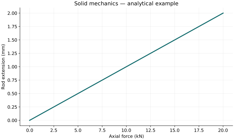
Definitions & inputs. F=10 kN,L=2 m,A=100 mm²,E=200 GPa.
Choose the governing model and isolate the requested quantity.
Insert the stated inputs in consistent units or the explicitly defined normalized units.
Evaluate the expression; the result uses the units shown.
Interpretation. The rod extends by one millimetre.
↑ Return to definitions and contentsExample 04. Lateral strain
Definitions & inputs. ν=.3, axial strain .001.
Choose the governing model and isolate the requested quantity.
Insert the stated inputs in consistent units or the explicitly defined normalized units.
Evaluate the expression; the result uses the units shown.
Interpretation. Positive axial extension produces lateral contraction.
↑ Return to definitions and contentsExample 05. Shear modulus
Definitions & inputs. E=210 GPa,ν=.3, isotropic material.
Choose the governing model and isolate the requested quantity.
Insert the stated inputs in consistent units or the explicitly defined normalized units.
Evaluate the expression; the result uses the units shown.
Interpretation. E, G and ν are not independent for isotropic elasticity.
↑ Return to definitions and contentsExample 06. Bulk modulus
Definitions & inputs. E=210 GPa,ν=.3.
Choose the governing model and isolate the requested quantity.
Insert the stated inputs in consistent units or the explicitly defined normalized units.
Evaluate the expression; the result uses the units shown.
Interpretation. K describes hydrostatic compression.
↑ Return to definitions and contentsExample 07. Circular shaft polar moment
Definitions & inputs. Radius r=10 mm.
Choose the governing model and isolate the requested quantity.
Insert the stated inputs in consistent units or the explicitly defined normalized units.
Evaluate the expression; the result uses the units shown.
Interpretation. Hollow shafts subtract the inner radius fourth power.
↑ Return to definitions and contentsExample 08. Shaft surface shear
Definitions & inputs. T=10 N m,r=.01 m,J=πr⁴/2.
Choose the governing model and isolate the requested quantity.
Insert the stated inputs in consistent units or the explicitly defined normalized units.
Evaluate the expression; the result uses the units shown.
Interpretation. Maximum shear occurs at the outer radius.
↑ Return to definitions and contentsExample 09. Shaft twist
Definitions & inputs. T=10 N m,L=1 m,G=80 GPa,J=π(0.01)⁴/2.
Choose the governing model and isolate the requested quantity.
Insert the stated inputs in consistent units or the explicitly defined normalized units.
Evaluate the expression; the result uses the units shown.
Interpretation. This omits end effects near torque introduction.
↑ Return to definitions and contentsExample 10. Rectangular beam area moment
Definitions & inputs. Width b=.02 m,height h=.04 m.
Choose the governing model and isolate the requested quantity.
Insert the stated inputs in consistent units or the explicitly defined normalized units.
Evaluate the expression; the result uses the units shown.
Interpretation. Height is measured along the bending direction.
↑ Return to definitions and contentsExample 11. Bending surface stress
Definitions & inputs. M=100 N m,y=.02 m,I=1.0666667×10⁻⁷ m⁴.
Choose the governing model and isolate the requested quantity.
Insert the stated inputs in consistent units or the explicitly defined normalized units.
Evaluate the expression; the result uses the units shown.
Interpretation. The opposite surface has the opposite stress sign.
↑ Return to definitions and contentsExample 12. Cantilever tip deflection
Definitions & inputs. F=10 N,L=.5 m,E=200 GPa,I=10⁻⁸ m⁴.
Choose the governing model and isolate the requested quantity.
Insert the stated inputs in consistent units or the explicitly defined normalized units.
Evaluate the expression; the result uses the units shown.
Interpretation. Valid while deflection and rotations remain small.
↑ Return to definitions and contentsExample 13. Simply supported midpoint moment
Definitions & inputs. Centre point load F=100 N,span L=2 m.
Choose the governing model and isolate the requested quantity.
Insert the stated inputs in consistent units or the explicitly defined normalized units.
Evaluate the expression; the result uses the units shown.
Interpretation. End supports transmit no bending moment in this model.
↑ Return to definitions and contentsExample 14. Elastic strain energy
Definitions & inputs. Final F=1000 N,linear extension δ=.001 m.
Choose the governing model and isolate the requested quantity.
Insert the stated inputs in consistent units or the explicitly defined normalized units.
Evaluate the expression; the result uses the units shown.
Interpretation. The result assumes loading from zero without dissipation.
↑ Return to definitions and contentsExample 15. Von Mises plane stress
Definitions & inputs. Principal stresses 100 and 50 MPa; third is zero.
Choose the governing model and isolate the requested quantity.
Insert the stated inputs in consistent units or the explicitly defined normalized units.
Evaluate the expression; the result uses the units shown.
Interpretation. Principal values already account for any shear transformation.
↑ Return to definitions and contentsExample 16. Yield ratio
Definitions & inputs. Yield strength 250 MPa, equivalent applied stress 100 MPa.
Choose the governing model and isolate the requested quantity.
Insert the stated inputs in consistent units or the explicitly defined normalized units.
Evaluate the expression; the result uses the units shown.
Interpretation. Other failure modes may control.
↑ Return to definitions and contentsExample 17. Free thermal elongation
Definitions & inputs. α=12×10⁻⁶/K,L=2 m,ΔT=50 K.
Choose the governing model and isolate the requested quantity.
Insert the stated inputs in consistent units or the explicitly defined normalized units.
Evaluate the expression; the result uses the units shown.
Interpretation. No mechanical load develops when expansion is unrestrained.
↑ Return to definitions and contentsExample 18. Fully restrained thermal stress
Definitions & inputs. E=200 GPa,α=12×10⁻⁶/K,ΔT=50 K.
Choose the governing model and isolate the requested quantity.
Insert the stated inputs in consistent units or the explicitly defined normalized units.
Evaluate the expression; the result uses the units shown.
Interpretation. Heating produces compression; yielding or buckling may invalidate the elastic result.
↑ Return to definitions and contentsExample 19. Pinned Euler column
Definitions & inputs. E=200 GPa,I=10⁻⁸ m⁴,L=1 m,K=1.
Choose the governing model and isolate the requested quantity.
Insert the stated inputs in consistent units or the explicitly defined normalized units.
Evaluate the expression; the result uses the units shown.
Interpretation. This is an ideal bifurcation load, not an allowable load.
↑ Return to definitions and contentsExample 20. Cantilever stiffness
Definitions & inputs. E=200 GPa,I=10⁻⁸ m⁴,L=.5 m.
Choose the governing model and isolate the requested quantity.
Insert the stated inputs in consistent units or the explicitly defined normalized units.
Evaluate the expression; the result uses the units shown.
Interpretation. This maps a small transverse tip displacement to tip force.
↑ Return to definitions and contentsSymbols and units
Each derivation and problem defines its own symbols and inputs. Symbols may be reused with different meanings in other subjects. Keep units consistent, retain sufficient precision during calculation, and apply the stated validity limits.