Astrophysics: from radiation to stars and galaxies

1. Infer distance and luminosity from observed light

Definitions & inputs. L is total luminosity (W), F received bolometric flux (W m⁻²), d distance, and p annual parallax angle. m and M are apparent and absolute magnitudes in the same photometric band.

1. Conservation spreads emitted power over a sphere; flux is power per collecting area, not total power.

   $$L=\int F\,dA=4\pi d^2F\quad\Rightarrow\quad F=\frac{L}{4\pi d^2}$$

2. For a small angle, the apparent displacement relative to the solar-system barycentre gives distance. Annual parallax is the semi-angle, not the full six-month displacement.

   $$p\simeq\frac{1\ {\rm AU}}d\ ({\rm radians}),\quad d({\rm pc})=\frac1{p({\rm arcsec})}$$

3. The magnitude scale is logarithmic: brighter objects have smaller magnitudes.

   $$m_1-m_2=-2.5\log_{10}(F_1/F_2)$$

4. Insert inverse-square flux into the magnitude difference. A is extinction in magnitudes in the chosen band.

   $$M=m(d=10\ {\rm pc}),\quad m-M=5\log_{10}[d/(10\ {\rm pc})]+A$$

Interpretation. Distance, extinction, and bolometric correction are separate inference steps. A band-limited flux is not automatically the bolometric flux used with total luminosity.

• OpenStax Astronomy — distances and stellar parallax ↗

2. Thermal spectra, stellar radius, and Doppler shifts

Definitions & inputs. Bλ is spectral radiance per wavelength per solid angle; T temperature; σSB the Stefan–Boltzmann constant; R radius; λ0 rest wavelength; vr radial velocity positive for recession.

1. Planck’s distribution combines photon mode density and Bose occupation. This is radiance per unit wavelength, not per unit frequency.

   $$B_\lambda(T)=\frac{2hc^2}{\lambda^5}\frac1{e^{hc/(\lambda k_BT)}-1}$$

2. Integrate over the outward hemisphere and wavelength, then multiply by the stellar surface area. Effective temperature is defined by this luminosity relation.

   $$F_{\rm surface}=\int_0^\infty\pi B_\lambda d\lambda=\sigma_{\rm SB}T^4,\quad L=4\pi R^2\sigma_{\rm SB}T_{\rm eff}^4$$

3. Set ∂Bλ/∂λ=0. The nonzero root x≈4.96511 yields Wien’s displacement law; the Bν peak is at a different location.

   $$x=hc/(\lambda k_BT),\quad5(1-e^{-x})=x,\quad\lambda_{\max}T=2.897771955\times10^{-3}\ {\rm m\,K}$$

4. A small nonrelativistic Doppler shift gives line-of-sight velocity. Gravitational and cosmological redshifts require their own interpretation.

   $$z=\frac{\lambda_{\rm obs}-\lambda_0}{\lambda_0}\simeq\frac{v_r}{c}\quad(|v_r|\ll c)$$

Interpretation. Combining distance, luminosity, color, and spectroscopy constrains stars, but each inference retains model assumptions.

• OpenStax Astronomy — blackbody radiation and radiation laws ↗

3. Infer masses from orbital dynamics

Definitions & inputs. M1,M2 are two masses, a is the semimajor axis of their relative separation, P orbital period, and i inclination. G is Newton’s constant.

1. Subtract the two body equations of motion to obtain the relative orbit.

   $$\ddot{\mathbf r}=-\frac{G(M_1+M_2)}{r^3}\mathbf r$$

2. For a circular orbit, equate centripetal and gravitational acceleration. The same Kepler law holds for an elliptical orbit with semimajor axis a.

   $$\text{circular: }\frac{4\pi^2a}{P^2}=\frac{G(M_1+M_2)}{a^2}\Rightarrow P^2=\frac{4\pi^2a^3}{G(M_1+M_2)}$$

3. The centre-of-mass condition relates the two orbital sizes.

   $$M_1a_1=M_2a_2,\quad a=a_1+a_2$$

4. The primary’s radial-velocity semiamplitude includes eccentricity e and inclination. It does not alone determine the companion mass without other information.

   $$K_1=\frac{2\pi a_1\sin i}{P\sqrt{1-e^2}}$$

Interpretation. Use the relative separation for a, not one component’s distance from the centre of mass.

• OpenStax Astronomy — measuring stellar masses ↗

4. Derive the equations of stellar structure

Definitions & inputs. Mr is mass enclosed within radius r, ρ density, P total pressure, Lr outward luminosity, ε net local energy generation per unit mass (W kg⁻¹), and κR Rosseland mean opacity (m² kg⁻¹).

1. A thin spherical shell has volume 4πr²dr.

   $$dM_r=4\pi r^2\rho\,dr\Rightarrow\frac{dM_r}{dr}=4\pi r^2\rho$$

2. Balance the shell’s pressure force against gravity; pressure decreases outward.

   $$4\pi r^2dP=-\frac{GM_r}{r^2}dM_r\Rightarrow\frac{dP}{dr}=-\frac{GM_r\rho}{r^2}$$

3. Local energy production changes the luminosity passing through each shell. Time-dependent thermal evolution adds entropy terms.

   $$dL_r=\epsilon\,dM_r\Rightarrow\frac{dL_r}{dr}=4\pi r^2\rho\epsilon$$

4. In optically thick radiative diffusion, insert F=Lr/(4πr²). A convective zone needs a different heat-transport prescription.

   $$F_{\rm rad}=-\frac{16\sigma_{\rm SB}T^3}{3\kappa_R\rho}\frac{dT}{dr},\quad\frac{dT}{dr}=-\frac{3\kappa_R\rho L_r}{64\pi\sigma_{\rm SB}r^2T^3}$$

5. Illustrative ideal-gas and radiation terms depend on mean particle mass μmp. Degeneracy or strong interactions require other equations of state.

   $$P_{\rm gas}=\frac{\rho k_BT}{\mu m_p},\quad P_{\rm rad}=\frac{4\sigma_{\rm SB}}{3c}T^4$$

Interpretation. Hydrostatic balance is not thermal balance. These coupled equations must normally be integrated numerically rather than replaced by one uniform-density estimate.

• Princeton Astrophysics — stellar structure, virial theorem, transfer, and timescales ↗

5. Virial balance and stellar energy timescales

Definitions & inputs. Ω is negative gravitational potential energy, U internal energy, N particle count, μ mean molecular weight in proton-mass units, and L luminosity.

1. Multiply hydrostatic balance by 4πr³dr and recognize the gravitational binding-energy integral.

   $$\int_0^R4\pi r^3\frac{dP}{dr}dr=-\int_0^M\frac{GM_r}{r}dM_r=\Omega$$

2. Integrate the left side by parts; discard surface pressure only under the stated assumption.

   $$4\pi R^3P(R)-3\int P\,dV=\Omega,\quad P(R)\simeq0\Rightarrow3\int P\,dV+\Omega=0$$

3. For a monatomic ideal gas, gravitational contraction makes the total energy more negative while raising internal energy.

   $$U=\tfrac32\int P\,dV\Rightarrow2U+\Omega=0,\quad E=U+\Omega=\Omega/2$$

4. Insert the uniform-sphere binding energy and U=3NkB⟨T⟩/2 with N=M/(μmp). This is a particle-weighted mean temperature, not the central temperature.

   $$\rho=\text{constant}:\quad\Omega=-\frac{3GM^2}{5R},\quad\langle T\rangle=\frac{GM\mu m_p}{5k_BR}$$

5. The first is a gravitational energy-scale estimate; the second uses burned hydrogen mass fraction fH and conversion efficiency η. Neither assumes L remains constant in a realistic evolution calculation.

   $$t_{\rm KH}\sim\frac{GM^2}{RL},\quad t_{\rm fuel}\sim\frac{\eta f_HMc^2}{L}$$

Interpretation. Nuclear fuel can sustain luminosity much longer than gravitational contraction alone. Dense stellar remnants require quantum equations of state and sometimes GR.

• Princeton Astrophysics — stellar structure, virial theorem, transfer, and timescales ↗

6. Radiative transfer, optical depth, and the Eddington scale

Definitions & inputs. Iν is specific intensity; αν absorption coefficient (m⁻¹); jν emission coefficient; κ is a flux-mean mass opacity; τ is optical depth; Sν=jν/αν is the source function.

1. Along the propagation direction absorption removes intensity and emission adds it.

   $$\frac{dI_\nu}{ds}=-\alpha_\nu I_\nu+j_\nu,\quad d\tau_\nu=\alpha_\nu ds$$

2. For constant source function, solve the first-order equation with an integrating factor. Pure attenuation sets Sν=0.

   $$\frac{dI_\nu}{d\tau_\nu}=-I_\nu+S_\nu\Rightarrow I_\nu(\tau)=I_\nu(0)e^{-\tau}+S_\nu(1-e^{-\tau})$$

3. Radiation carries momentum flux F/c; multiply by opacity per unit mass to get acceleration.

   $$a_{\rm rad}=\kappa F/c=\frac{\kappa L}{4\pi r^2c},\quad a_g=GM/r^2$$

4. Balance the two accelerations. Radius cancels for spherical inverse-square flux.

   $$a_{\rm rad}=a_g\Rightarrow L_{\rm Edd}=\frac{4\pi GMc}{\kappa}$$

Interpretation. The Eddington luminosity is a model-dependent force-balance scale, not an absolute brightness limit for every source geometry.

• Princeton Astrophysics — stellar structure, virial theorem, transfer, and timescales ↗

7. Gas-cloud collapse: free-fall time and Jeans instability

Definitions & inputs. ρ0 is background mass density, cs is isothermal sound speed, k perturbation wave number, and ω its frequency. μmp is the mean particle mass.

1. Integrate energy conservation for a shell released from rest; use M=4πρ0R³/3. This is a pressureless dynamical time, not a universal star-formation time.

   $$\dot r^2=2GM(1/r-1/R),\quad t_{\rm ff}=\int_0^R\frac{dr}{\sqrt{2GM(1/r-1/R)}}=\sqrt{\frac{3\pi}{32G\rho_0}}$$

2. Linearize continuity, momentum balance, and Poisson’s equation about the chosen background.

   $$\partial_t\delta\rho+\rho_0\nabla\cdot\delta\mathbf v=0,\quad\partial_t\delta\mathbf v=-\frac{c_s^2}{\rho_0}\nabla\delta\rho-\nabla\delta\Phi,\quad\nabla^2\delta\Phi=4\pi G\delta\rho$$

3. Eliminate velocity and potential, then substitute a plane wave. Negative ω² indicates exponential growth.

   $$\partial_t^2\delta\rho=c_s^2\nabla^2\delta\rho+4\pi G\rho_0\delta\rho\Rightarrow\omega^2=c_s^2k^2-4\pi G\rho_0$$

4. The zero-frequency boundary defines the Jeans wavelength. Here Jeans mass means the mass within a sphere of radius λJ/2; other conventions have different factors.

   $$c_s=\sqrt{\frac{k_BT}{\mu m_p}},\quad\lambda_J=c_s\sqrt{\frac\pi{G\rho_0}},\quad M_J=\frac{4\pi}3\rho_0(\lambda_J/2)^3$$

Interpretation. Magnetic support, rotation, turbulent pressure, cooling, and geometry change collapse thresholds. Define the mass convention before comparing values.

• Tong — Cosmology: Jeans instability and structure formation ↗

8. Planet transits and orbital inference

Definitions & inputs. Rp and R★ are planet and stellar radii; δ is the fractional flux loss; a orbital semimajor axis; P period; b transit impact parameter in stellar-radius units.

1. Divide blocked projected area by the stellar disk area.

   $$F_{\rm blocked}\propto\pi R_p^2,\quad F_\star\propto\pi R_\star^2\Rightarrow\delta=(R_p/R_\star)^2$$

2. A transit measures a radius ratio; absolute planet radius inherits uncertainty in the star’s radius.

   $$R_p=R_\star\sqrt\delta$$

3. Repeated transits determine period; a stellar mass model then converts it to an orbital scale.

   $$M_p\ll M_\star:\quad a=\left(\frac{GM_\star P^2}{4\pi^2}\right)^{1/3}$$

4. Viewing geometry controls whether a transit occurs and its chord length. A shallow dip alone does not uniquely establish a planet.

   $$b=\frac{a\cos i}{R_\star}\quad(\text{circular orbit})$$

Interpretation. Spectroscopy, stellar characterization, multiple transits, and false-positive checks complement the simplified area model.

• NASA — Exoplanet Watch: transit depth and observational definitions ↗

9. Galaxies, dynamical mass, and the cosmic distance connection

Definitions & inputs. v is circular speed at radius r, M(<r) enclosed mass, H0 a chosen present expansion rate, z cosmological redshift, and dL luminosity distance.

1. Balance centripetal and gravitational acceleration. Disks require their actual gravitational geometry for accurate mass inference.

   $$v^2/r=GM(<r)/r^2\Rightarrow M(<r)=v^2r/G$$

2. A flat rotation curve does not match a finite central point mass whose Keplerian speed decreases as r⁻¹/².

   $$v\simeq\text{constant}\Rightarrow M(<r)\propto r$$

3. Low-redshift recession offers an approximate distance estimate. The luminosity-distance definition retains inverse-square notation while incorporating expansion effects.

   $$cz\simeq H_0d\quad(z\ll1),\qquad F=L/(4\pi d_L^2)$$

4. At larger redshift, integrate the expansion history. This expression assumes spatial flatness and standard photon propagation.

   $$\text{flat FLRW:}\quad d_L(z)=(1+z)c\int_0^z\frac{dz^\prime}{H(z^\prime)}$$

Interpretation. Astrophysical observations constrain models rather than directly measuring all intrinsic properties. Geometry, dust, selection effects, and calibration propagate into the result.

• OpenStax Astronomy — dynamical mass of the Galaxy ↗
• Tong — General Relativity: Einstein equations and matter ↗

Twenty worked astrophysics examples

Inputs are illustrative reference values, not current catalog measurements. Solar reference values used here are M⊙=1.98847×10³⁰ kg, R⊙=6.957×10⁸ m, and L⊙=3.828×10²⁶ W. One Julian year is 365.25 days. Each example links to its governing derivation.

Example 01. Distance from a 25-milliarcsecond parallax

Definitions & inputs. Annual parallax p=25 mas.

Review the governing derivation ↑

1. Convert milliarcseconds to arcseconds.

   $$p=25\ {\rm mas}=0.025\ {\rm arcsec}$$

2. Invert the angle in the parsec definition.

   $$d=1/p=1/0.025=40.0\ {\rm pc}$$

3. Convert to SI distance.

   $$d=40(3.08567758\times10^{16})=1.23427e+18\ {\rm m}$$

Interpretation. If parallax uncertainty is large, direct inversion can be a biased distance estimator.

• OpenStax Astronomy — distances and stellar parallax ↗

Example 02. Flux of a solar-luminosity star at 10 pc

Definitions & inputs. L=3.828×10²⁶ W; d=10 pc.

Review the governing derivation ↑

1. Convert distance to metres.

   $$d=10\ {\rm pc}=3.08567758\times10^{17}\ {\rm m}$$

2. Divide emitted power by the sphere’s area.

   $$F=L/(4\pi d^2)$$

3. This is the total energy flux integrated over wavelength.

   $$F=3.19934e-10\ {\rm W\,m^{-2}}$$

Interpretation. At twice the distance the flux falls to one quarter.

• OpenStax Astronomy — distances and stellar parallax ↗

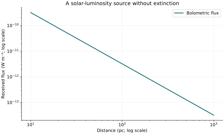
Example 03. Distance from apparent and absolute magnitudes

Definitions & inputs. m=10.0, M=5.0, extinction A=0.0 in the same band.

Review the governing derivation ↑

1. Insert the observed and intrinsic magnitudes.

   $$m-M-A=5=5\log_{10}[d/(10\ {\rm pc})]$$

2. Divide the modulus by five.

   $$\log_{10}[d/(10\ {\rm pc})]=1$$

3. Exponentiate and restore the ten-parsec normalization.

   $$d=10\times10^1=100\ {\rm pc}$$

Interpretation. Positive uncorrected extinction would make this inferred distance too large.

• OpenStax Astronomy — distances and stellar parallax ↗

Example 04. Temperature from a wavelength-spectrum peak

Definitions & inputs. A blackbody Bλ spectrum peaks at λmax=500 nm.

Review the governing derivation ↑

1. Convert the wavelength.

   $$\lambda_{\max}=500\ {\rm nm}=5.00\times10^{-7}\ {\rm m}$$

2. Use the nonzero Planck-peak solution.

   $$T=b/\lambda_{\max},\quad b=2.897771955\times10^{-3}\ {\rm m\,K}$$

3. Divide the displacement constant by the wavelength.

   $$T=5795.54\ {\rm K}$$

Interpretation. A Bν peak cannot be substituted into this wavelength formula.

• OpenStax Astronomy — blackbody radiation and radiation laws ↗

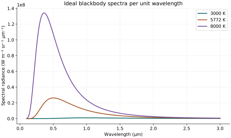
Example 05. Radius from luminosity and temperature

Definitions & inputs. L=4L⊙, Teff=5772 K; σSB=5.670374419×10⁻⁸ SI.

Review the governing derivation ↑

1. Isolate radius before substituting.

   $$L=4\pi R^2\sigma_{\rm SB}T_{\rm eff}^4\Rightarrow R=\sqrt{L/(4\pi\sigma_{\rm SB}T_{\rm eff}^4)}$$

2. Evaluate with the stated bolometric luminosity.

   $$R=\sqrt{4(3.828\times10^{26})/(4\pi\sigma_{\rm SB}5772^4)}=1.3914e+09\ {\rm m}$$

3. Compare with R⊙=6.957×10⁸ m.

   $$R/R_\odot=2$$

Interpretation. At fixed temperature, radius scales as the square root of luminosity.

• OpenStax Astronomy — blackbody radiation and radiation laws ↗

Example 06. Radial velocity from an absorption-line shift

Definitions & inputs. λ0=656.28 nm and λobs=656.50 nm.

Review the governing derivation ↑

1. Compute the redward shift.

   $$\Delta\lambda=656.50-656.28=0.22\ {\rm nm}$$

2. Form a dimensionless fractional shift.

   $$z=\Delta\lambda/\lambda_0=0.22/656.28$$

3. A positive value means recession under this convention.

   $$v_r\simeq cz=100.497\ {\rm km\,s^{-1}}$$

Interpretation. Instrumental, gravitational, and atmospheric line shifts must be separated in precision work.

• OpenStax Astronomy — blackbody radiation and radiation laws ↗

Example 07. Total mass of a resolved binary

Definitions & inputs. Relative-orbit semimajor axis a=2 AU; period P=2 Julian years.

Review the governing derivation ↑

1. Rearrange Kepler’s third law.

   $$M_1+M_2=4\pi^2a^3/(GP^2)$$

2. Use consistent SI units.

   $$a=2(1.495978707\times10^{11})\ {\rm m},\quad P=2(365.25)(86400)\ {\rm s}$$

3. Evaluate and divide by the stated solar mass.

   $$M_{\rm tot}=2.00002\ M_\odot$$

Interpretation. The total mass does not by itself specify the individual masses.

• OpenStax Astronomy — measuring stellar masses ↗

Example 08. Orbital scale for a ten-day planet

Definitions & inputs. P=10 days, M★=M⊙, Mp≪M★.

Review the governing derivation ↑

1. Convert the measured repeat period.

   $$P=10(86400)=864000\ {\rm s}$$

2. Solve Kepler’s law for semimajor axis.

   $$a=[GM_\star P^2/(4\pi^2)]^{1/3}$$

3. Express the result in astronomical units.

   $$a=0.0908389\ {\rm AU}$$

Interpretation. An orbital period gives an orbital scale only after specifying the host mass.

• OpenStax Astronomy — measuring stellar masses ↗

Example 09. Mean density of a solar-size star

Definitions & inputs. M=M⊙=1.98847×10³⁰ kg; R=R⊙=6.957×10⁸ m.

Review the governing derivation ↑

1. Compute the sphere’s volume.

   $$V=4\pi R^3/3$$

2. Divide total mass by volume.

   $$\bar\rho=M/V=3M/(4\pi R^3)$$

3. The interior density varies greatly even though the mean is modest.

   $$\bar\rho=1409.82\ {\rm kg\,m^{-3}}$$

Interpretation. Do not use the mean density as a central density.

• Princeton Astrophysics — stellar structure, virial theorem, transfer, and timescales ↗

Example 10. Surface gravity of a solar-size star

Definitions & inputs. M=M⊙, R=R⊙.

Review the governing derivation ↑

1. Cancel the test mass.

   $$F_g=GMm/R^2\Rightarrow g=F_g/m=GM/R^2$$

2. Substitute the solar reference values.

   $$g=274.208\ {\rm m\,s^{-2}}$$

3. Convert to cgs before computing the spectroscopic log g convention.

   $$\log_{10}[g/({\rm cm\,s^{-2}})]=4.43808$$

Interpretation. log g is conventionally quoted using centimetres per second squared.

• Princeton Astrophysics — stellar structure, virial theorem, transfer, and timescales ↗

Example 11. Central pressure of a uniform-density sphere

Definitions & inputs. Toy sphere: M=M⊙ and R=R⊙; set P(R)=0 and ρ constant.

Review the governing derivation ↑

1. Insert the uniform enclosed mass into hydrostatic balance.

   $$M_r=4\pi\rho r^3/3,\quad dP/dr=-(4\pi G\rho^2/3)r$$

2. Integrate inward from the zero-pressure surface.

   $$P(r)=\frac{2\pi G\rho^2}{3}(R^2-r^2)$$

3. Replace density by 3M/(4πR³).

   $$P_c=\frac{2\pi G\rho^2R^2}{3}=\frac{3GM^2}{8\pi R^4}$$

4. Evaluate the benchmark central pressure.

   $$P_c=1.34474e+14\ {\rm Pa}$$

Interpretation. This is not the actual solar central pressure; it is a useful hydrostatic solver test.

• Princeton Astrophysics — stellar structure, virial theorem, transfer, and timescales ↗

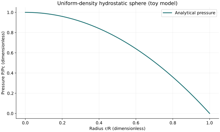
Example 12. Virial mean temperature of a toy star

Definitions & inputs. M=M⊙, R=R⊙, mean molecular weight μ=0.61.

Review the governing derivation ↑

1. Express internal energy using the number of freely moving particles.

   $$2U+\Omega=0,\quad U=\tfrac32(M/\mu m_p)k_B\langle T\rangle$$

2. Substitute the uniform-sphere binding energy and solve.

   $$\Omega=-3GM^2/(5R)\Rightarrow\langle T\rangle=GM\mu m_p/(5k_BR)$$

3. Evaluate the particle-weighted mean estimate.

   $$\langle T\rangle=2.81953e+06\ {\rm K}$$

Interpretation. This temperature is not a prediction of the Sun’s central temperature.

• Princeton Astrophysics — stellar structure, virial theorem, transfer, and timescales ↗

Example 13. Gravitational contraction timescale

Definitions & inputs. M=M⊙, R=R⊙, L=L⊙.

Review the governing derivation ↑

1. Divide the gravitational energy scale by the radiated power.

   $$E_g\sim GM^2/R,\quad t_{\rm KH}\sim E_g/L$$

2. Evaluate in seconds.

   $$t_{\rm KH}=9.90946e+14\ {\rm s}$$

3. Convert to million Julian years.

   $$t_{\rm KH}=31.4012\ {\rm Myr}$$

Interpretation. For a uniform ideal-gas sphere, the available total binding energy introduces a 3/10 factor; this conventional scale deliberately omits it.

• Princeton Astrophysics — stellar structure, virial theorem, transfer, and timescales ↗

Example 14. Hydrogen-burning energy-budget timescale

Definitions & inputs. M=M⊙, L=L⊙, burned hydrogen mass fraction fH=0.10 of total initial mass, η=0.007.

Review the governing derivation ↑

1. Define the fuel fraction as hydrogen actually burned, not a separate core fraction to be multiplied again.

   $$M_{H,\rm burned}=f_HM=0.10M$$

2. Use the approximate hydrogen-to-helium conversion efficiency.

   $$E_{\rm fuel}=\eta f_HMc^2=0.0007Mc^2$$

3. Convert the resulting energy-budget time to billions of years.

   $$t_{\rm fuel}=E_{\rm fuel}/L=10.3558\ {\rm Gyr}$$

Interpretation. This is a fuel-budget estimate, not a stellar-evolution track.

• Princeton Astrophysics — stellar structure, virial theorem, transfer, and timescales ↗

Example 15. Eddington scale for ten solar masses

Definitions & inputs. M=10M⊙ and prescribed opacity κ=0.034 m² kg⁻¹.

Review the governing derivation ↑

1. Write the outward and inward accelerations.

   $$a_{\rm rad}=\kappa L/(4\pi r^2c),\quad a_g=GM/r^2$$

2. Cancel radius and solve for luminosity.

   $$a_{\rm rad}=a_g\Rightarrow L_{\rm Edd}=4\pi GMc/\kappa$$

3. Evaluate the force-balance luminosity.

   $$L_{\rm Edd}=1.47054e+32\ {\rm W}=384153L_\odot$$

Interpretation. Opacity and emission geometry change the applicable luminosity scale.

• Princeton Astrophysics — stellar structure, virial theorem, transfer, and timescales ↗

Example 16. Transmission through optical depth two

Definitions & inputs. Incident intensity I0; optical depth τ=2.0; source function S=0.

Review the governing derivation ↑

1. Separate and integrate the transfer equation.

   $$dI/d\tau=-I\Rightarrow\int_{I_0}^{I}dI^\prime/I^\prime=-\tau$$

2. Only about 13.5% is transmitted.

   $$I/I_0=e^{-2}=0.135335$$

3. Convert the same attenuation into magnitudes.

   $$A=-2.5\log_{10}(I/I_0)=\frac{2.5}{\ln10}\tau=2.17147\ {\rm mag}$$

Interpretation. A nonzero source function or scattered light would change the observed intensity.

• Princeton Astrophysics — stellar structure, virial theorem, transfer, and timescales ↗

Example 17. Free-fall time of a molecular-cloud parcel

Definitions & inputs. Total particle number density n=10⁹ m⁻³ (10³ cm⁻³), mean particle mass μmp with μ=2.33.

Review the governing derivation ↑

1. Convert number density to mass density.

   $$\rho=\mu m_pn=2.33m_p(10^9)$$

2. Use the integrated pressureless collapse time.

   $$t_{\rm ff}=\sqrt{3\pi/(32G\rho)}$$

3. Convert seconds to million years.

   $$t_{\rm ff}=1.06629\ {\rm Myr}$$

Interpretation. Pressure, magnetic fields, or turbulence can delay or prevent collapse.

• Tong — Cosmology: Jeans instability and structure formation ↗

Example 18. Jeans mass of a ten-kelvin gas cloud

Definitions & inputs. T=10 K, μ=2.33, n=10⁹ m⁻³; ρ=μmpn.

Review the governing derivation ↑

1. Calculate thermal sound speed, not the adiabatic value with an extra γ factor.

   $$c_s=\sqrt{k_BT/(\mu m_p)}=188.22\ {\rm m\,s^{-1}}$$

2. Set ω²=0 in the dispersion relation.

   $$\lambda_J=c_s\sqrt{\pi/(G\rho)}=0.670362\ {\rm pc}$$

3. Compute the mass using the stated radius convention.

   $$M_J=\frac{4\pi}3\rho(\lambda_J/2)^3=9.08267\ M_\odot$$

Interpretation. Jeans mass scales as T^(3/2)ρ^(−1/2) at fixed composition; it is not a universal observed core mass.

• Tong — Cosmology: Jeans instability and structure formation ↗

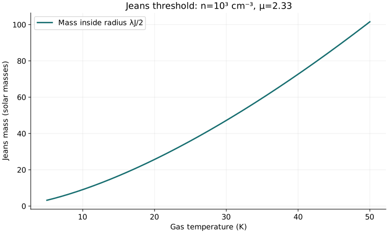
Example 19. Planet radius from a one-percent transit

Definitions & inputs. Transit depth δ=0.0100, stellar radius R★=R⊙.

Review the governing derivation ↑

1. Take the square root of the area ratio.

   $$\delta=(R_p/R_\star)^2\Rightarrow R_p/R_\star=\sqrt{0.0100}=0.100$$

2. Convert the inferred radius to kilometres.

   $$R_p=0.100R_\odot=69570\ {\rm km}$$

3. For independent small uncertainties, propagate logarithmic errors; the stellar radius can dominate.

   $$\frac{\sigma_{R_p}}{R_p}\simeq\sqrt{(\sigma_{R_\star}/R_\star)^2+\tfrac14(\sigma_\delta/\delta)^2}$$

Interpretation. A one-percent drop does not imply a one-percent radius ratio.

• NASA — Exoplanet Watch: transit depth and observational definitions ↗

Example 20. Enclosed mass from a circular speed

Definitions & inputs. v=200 km s⁻¹ at r=10 kpc.

Review the governing derivation ↑

1. Convert the measured scales.

   $$v=2.00\times10^5\ {\rm m\,s^{-1}},\quad r=10^4\ {\rm pc}$$

2. Use circular force balance.

   $$M(<r)=v^2r/G$$

3. Evaluate the dynamical mass within the specified radius.

   $$M(<r)=9.30006e+10\ M_\odot$$

Interpretation. This estimates total gravitating mass under the model; separating stars, gas, and dark matter requires independent information.

• OpenStax Astronomy — dynamical mass of the Galaxy ↗

Astrophysics brings the physics chapters together

• Quantum mechanics: atomic transitions, ionization, degeneracy, and nuclear microphysics supply spectra and equations of state.
• Quantum field theory: photon statistics and particle interactions underlie radiative processes; effective many-body models describe matter in suitable regimes.
• Solids and liquids: dust, rocky planets, icy bodies, and planetary interiors need material and phase models.
• Gases and plasmas: molecular clouds, atmospheres, stellar interiors, and ionized accretion flows require different kinetic, fluid, and magnetic approximations.
• General relativity: use relativistic gravity for compact objects, strong lensing, gravitational waves, and cosmology; the Newtonian benchmarks here have restricted regimes.

Numerical Modeling supplies methods for stellar ODE boundary-value problems, radiative transfer, gravitational N-body motion, and fluid or magnetohydrodynamic PDEs. The analytical examples here provide useful checks on those calculations.

Typical sensors and experimental connections

CCD image sensor · Spectrometer sensor · Bolometer / microbolometer

These are examples of instruments used to measure relevant observables, calibrate parameters, or test a physical system. They do not directly measure every abstract model quantity or prove a theory by themselves. Choose bandwidth, range, environment and uncertainty for the actual experiment.

Explore the dedicated Sensors site →

Mathematical tools and foundations

Derivatives and chain rule · Linear systems and elimination · Monte Carlo estimation

Use the stated mathematical conditions together with the physical assumptions. Explore the Mathematics atlas →