PHYSICS / ENGINEERING / COMPUTING
Optimization models and methods
Derive unconstrained minima, gradients, constrained optima and least-squares estimation through twenty worked examples.
Matter pathway: atom → solid → liquid → gas → plasma. Quantum mechanics and quantum field theory provide foundations across the pathway; they are not additional phases. This is a connected modeling route, not a universal heating curve. Actual phases depend on pressure, composition, and kinetics.
1. Stationarity and curvature
Definitions & inputs. f objective,x decision vector,g gradient,H Hessian.
Taylor expansion describes local slope and curvature.
A differentiable interior optimum must have zero first variation.
Positive curvature raises the objective for all small nonzero directions.
Interpretation. Convexity promotes a local optimum to global; zero gradient alone is insufficient.
↑ Return to definitions and contents2. Gradient and Newton steps
Definitions & inputs. α step length,g gradient,H invertible Hessian.
Move against local slope.
Minimize the local quadratic model for a Newton direction.
The quadratic error update has factors 1−αλ; bound their magnitude below one.
Interpretation. Nonconvex or ill-conditioned problems need safeguards; Newton is not globally convergent by default.
↑ Return to definitions and contents3. Constraints and KKT
Definitions & inputs. g_i(x)≤0 inequalities,h(x)=0 equalities,λi nonnegative multipliers,ν equality multiplier.
Add weighted constraints to form the Lagrangian.
Combine stationarity with primal and dual feasibility.
Complementarity says a slack inequality has zero multiplier.
Interpretation. Sign conventions for constraints determine multiplier signs; infeasible stationary points are not solutions.
↑ Return to definitions and contents4. Least squares and regularization
Definitions & inputs. A design matrix,b observations,x unknowns,λ nonnegative penalty.
Penalize the sum of squared residuals.
Differentiate with respect to the fitted coefficients.
Add λ‖x‖²/2 for ridge regularization.
Interpretation. QR or SVD is often numerically preferable to explicitly forming normal equations.
↑ Return to definitions and contentsGraphical worked example
Twenty worked examples
Open a problem to see its defined inputs, assumptions, equation, numerical substitution, result, and interpretation. Values are illustrative analytical exercises.
Example 01. Quadratic minimizer
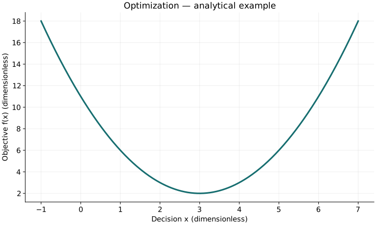
Definitions & inputs. f(x)=(x−3)²+2.
Choose the governing model and isolate the requested quantity.
Insert the stated inputs in consistent units or the explicitly defined normalized units.
Evaluate the expression; the result uses the units shown.
Interpretation. Positive second derivative 2 confirms a unique global minimum.
↑ Return to definitions and contentsExample 02. Minimum objective
Definitions & inputs. f(x)=(x−3)²+2,at x*=3.
Choose the governing model and isolate the requested quantity.
Insert the stated inputs in consistent units or the explicitly defined normalized units.
Evaluate the expression; the result uses the units shown.
Interpretation. Decision value and objective value are different quantities.
↑ Return to definitions and contentsExample 03. Gradient at a point
Definitions & inputs. f(x)=x²,x=4.
Choose the governing model and isolate the requested quantity.
Insert the stated inputs in consistent units or the explicitly defined normalized units.
Evaluate the expression; the result uses the units shown.
Interpretation. Units of the gradient are objective units per decision unit.
↑ Return to definitions and contentsExample 04. One gradient step
Definitions & inputs. f=x²,x0=4,α=.1.
Choose the governing model and isolate the requested quantity.
Insert the stated inputs in consistent units or the explicitly defined normalized units.
Evaluate the expression; the result uses the units shown.
Interpretation. The new objective is smaller than the initial value.
↑ Return to definitions and contentsExample 05. Gradient contraction
Definitions & inputs. f=x²,α=.1.
Choose the governing model and isolate the requested quantity.
Insert the stated inputs in consistent units or the explicitly defined normalized units.
Evaluate the expression; the result uses the units shown.
Interpretation. The decision error contracts by 0.8 per step in this quadratic.
↑ Return to definitions and contentsExample 06. Ten gradient steps
Definitions & inputs. Same quadratic,x0=4,r=.8.
Choose the governing model and isolate the requested quantity.
Insert the stated inputs in consistent units or the explicitly defined normalized units.
Evaluate the expression; the result uses the units shown.
Interpretation. The minimum is approached asymptotically for this step length.
↑ Return to definitions and contentsExample 07. Quadratic step upper bound
Definitions & inputs. f=x²/2,Hessian L=1.
Choose the governing model and isolate the requested quantity.
Insert the stated inputs in consistent units or the explicitly defined normalized units.
Evaluate the expression; the result uses the units shown.
Interpretation. At the endpoint the iterates oscillate without convergence.
↑ Return to definitions and contentsExample 08. Newton step for quadratic
Definitions & inputs. f=(x−3)²,x0=0,g=−6,H=2.
Choose the governing model and isolate the requested quantity.
Insert the stated inputs in consistent units or the explicitly defined normalized units.
Evaluate the expression; the result uses the units shown.
Interpretation. Newton reaches this exact quadratic minimizer in one step.
↑ Return to definitions and contentsExample 09. Newton step for quartic
Definitions & inputs. f=x⁴,x0=2,g=32,H=48.
Choose the governing model and isolate the requested quantity.
Insert the stated inputs in consistent units or the explicitly defined normalized units.
Evaluate the expression; the result uses the units shown.
Interpretation. It does not reach the nonquadratic minimum in one step.
↑ Return to definitions and contentsExample 10. Projection onto interval
Definitions & inputs. Candidate x=3,feasible interval [0,2].
Choose the governing model and isolate the requested quantity.
Insert the stated inputs in consistent units or the explicitly defined normalized units.
Evaluate the expression; the result uses the units shown.
Interpretation. Projection minimizes Euclidean distance to the feasible interval.
↑ Return to definitions and contentsExample 11. Bound-constrained quadratic
Definitions & inputs. Minimize (x−3)² with x≤1.
Choose the governing model and isolate the requested quantity.
Insert the stated inputs in consistent units or the explicitly defined normalized units.
Evaluate the expression; the result uses the units shown.
Interpretation. The optimum lies at the active upper bound.
↑ Return to definitions and contentsExample 12. KKT multiplier
Definitions & inputs. Same objective and g=x−1≤0 at x*=1.
Choose the governing model and isolate the requested quantity.
Insert the stated inputs in consistent units or the explicitly defined normalized units.
Evaluate the expression; the result uses the units shown.
Interpretation. λ is nonnegative, satisfying dual feasibility.
↑ Return to definitions and contentsExample 13. Equality-constrained split
Definitions & inputs. Minimize x²+y² subject to x+y=10.
Choose the governing model and isolate the requested quantity.
Insert the stated inputs in consistent units or the explicitly defined normalized units.
Evaluate the expression; the result uses the units shown.
Interpretation. The other decision y is also 5.
↑ Return to definitions and contentsExample 14. Weighted resource split
Definitions & inputs. Minimize x²+4y² with x+y=10.
Choose the governing model and isolate the requested quantity.
Insert the stated inputs in consistent units or the explicitly defined normalized units.
Evaluate the expression; the result uses the units shown.
Interpretation. The corresponding x=8 gives lower penalty to the more expensive y component.
↑ Return to definitions and contentsExample 15. Least-squares constant
Definitions & inputs. Observations 2,4,6; fit one common value.
Choose the governing model and isolate the requested quantity.
Insert the stated inputs in consistent units or the explicitly defined normalized units.
Evaluate the expression; the result uses the units shown.
Interpretation. The residuals sum to zero.
↑ Return to definitions and contentsExample 16. Through-origin fitted slope
Definitions & inputs. x samples 1,2; y samples 2,5; fit y=ax.
Choose the governing model and isolate the requested quantity.
Insert the stated inputs in consistent units or the explicitly defined normalized units.
Evaluate the expression; the result uses the units shown.
Interpretation. An intercept was explicitly excluded.
↑ Return to definitions and contentsExample 17. Scalar ridge estimate
Definitions & inputs. Minimize (x−3)²/2+λx²/2 with λ=2.
Choose the governing model and isolate the requested quantity.
Insert the stated inputs in consistent units or the explicitly defined normalized units.
Evaluate the expression; the result uses the units shown.
Interpretation. Regularization shrinks the estimate toward zero.
↑ Return to definitions and contentsExample 18. Two-dimensional gradient norm
Definitions & inputs. Gradient components 3 and 4.
Choose the governing model and isolate the requested quantity.
Insert the stated inputs in consistent units or the explicitly defined normalized units.
Evaluate the expression; the result uses the units shown.
Interpretation. Convergence tolerances need scaling appropriate to variables and objective.
↑ Return to definitions and contentsExample 19. Small linear program
Definitions & inputs. Maximize 3x+2y with x,y≥0 and x+y≤4.
Choose the governing model and isolate the requested quantity.
Insert the stated inputs in consistent units or the explicitly defined normalized units.
Evaluate the expression; the result uses the units shown.
Interpretation. The upper bound is attained at x=4,y=0, proving optimality.
↑ Return to definitions and contentsExample 20. Quadratic condition number
Definitions & inputs. Positive Hessian eigenvalues 1 and 100.
Choose the governing model and isolate the requested quantity.
Insert the stated inputs in consistent units or the explicitly defined normalized units.
Evaluate the expression; the result uses the units shown.
Interpretation. Strong curvature anisotropy can slow unpreconditioned gradient descent.
↑ Return to definitions and contentsSymbols and units
Each derivation and problem defines its own symbols and inputs. Symbols may be reused with different meanings in other subjects. Keep units consistent, retain sufficient precision during calculation, and apply the stated validity limits.