PHYSICS / ENGINEERING / COMPUTING
Reliability calculation models
Distinguish lifetime reliability, failure distributions, redundancy, availability and statistical evidence through twenty worked examples.
Matter pathway: atom → solid → liquid → gas → plasma. Quantum mechanics and quantum field theory provide foundations across the pathway; they are not additional phases. This is a connected modeling route, not a universal heating curve. Actual phases depend on pressure, composition, and kinetics.
1. Lifetime and hazard
Definitions & inputs. T random lifetime,R(t) survival probability,F(t) failure CDF,f density,h hazard.
Hazard is a conditional instantaneous failure rate, not a probability by itself.
Differentiate survival and substitute the hazard definition.
Integrate with R(0)=1.
Interpretation. Constant hazard gives exponential survival; wearout and infant mortality do not generally have constant hazard.
↑ Return to definitions and contents2. Lifetime distributions
Definitions & inputs. λ constant hazard,η Weibull scale,β Weibull shape,MTTF expected lifetime.
Integrate exponential survival over time.
Differentiate the Weibull cumulative hazard.
Mean lifetime averages over the distribution; it is not a guaranteed life.
Interpretation. Weibull shape below, equal to, or above one represents decreasing, constant, or increasing hazard.
↑ Return to definitions and contents3. System structure
Definitions & inputs. Ri component survival at the same mission time; n identical units with reliability R.
All series components must survive.
Parallel success is the complement of all components failing.
Count mutually exclusive cases with two or three surviving units.
Interpretation. Common causes, load sharing, standby aging and imperfect switching invalidate simple independence formulas.
↑ Return to definitions and contents4. Repair and evidence
Definitions & inputs. MTBF mean operating time between failures,MTTR mean repair time,Ttest total exposure,α one-sided tail probability.
Long-run uptime fraction is mean up duration divided by the full cycle.
Poisson counting under a constant failure rate gives the zero-event likelihood.
Solve the zero-event probability for a one-sided upper rate bound.
Interpretation. A test bound is model-dependent statistical evidence; zero observed failures does not establish perfect reliability.
↑ Return to definitions and contentsGraphical worked example
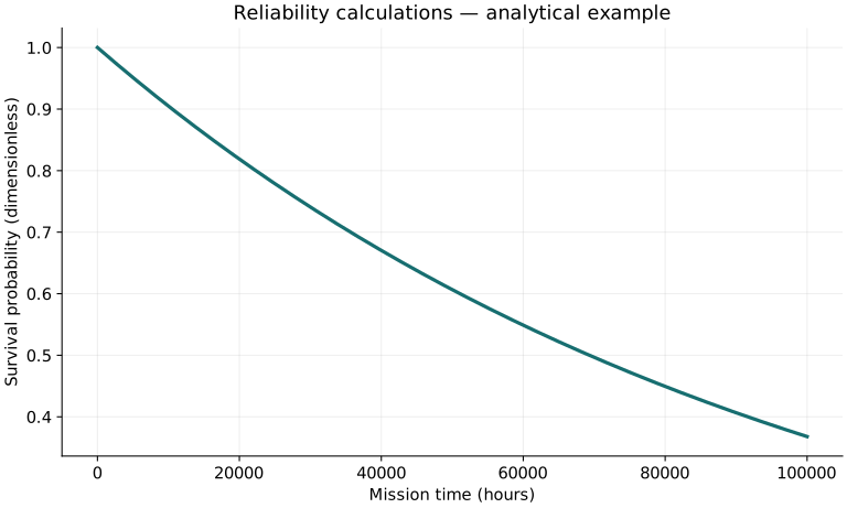
Twenty worked examples
Open a problem to see its defined inputs, assumptions, equation, numerical substitution, result, and interpretation. Values are illustrative analytical exercises.
Example 01. Exponential mission reliability
Definitions & inputs. λ=10⁻⁵/h,t=1000 h.
Choose the governing model and isolate the requested quantity.
Insert the stated inputs in consistent units or the explicitly defined normalized units.
Evaluate the expression; the result uses the units shown.
Interpretation. Constant hazard is assumed over this mission interval.
↑ Return to definitions and contentsExample 02. Mission failure probability
Definitions & inputs. Same λ=10⁻⁵/h,t=1000 h.
Choose the governing model and isolate the requested quantity.
Insert the stated inputs in consistent units or the explicitly defined normalized units.
Evaluate the expression; the result uses the units shown.
Interpretation. Reliability and failure probability sum to one.
↑ Return to definitions and contentsExample 03. Mean exponential life
Definitions & inputs. λ=2×10⁻⁵/h.
Choose the governing model and isolate the requested quantity.
Insert the stated inputs in consistent units or the explicitly defined normalized units.
Evaluate the expression; the result uses the units shown.
Interpretation. This is a mean, not a lower guaranteed lifetime.
↑ Return to definitions and contentsExample 04. Median exponential life
Definitions & inputs. λ=2×10⁻⁵/h.
Choose the governing model and isolate the requested quantity.
Insert the stated inputs in consistent units or the explicitly defined normalized units.
Evaluate the expression; the result uses the units shown.
Interpretation. Half of the modeled population survives past the median.
↑ Return to definitions and contentsExample 05. Required hazard for target
Definitions & inputs. R≥.99 over 1000 h,exponential model.
Choose the governing model and isolate the requested quantity.
Insert the stated inputs in consistent units or the explicitly defined normalized units.
Evaluate the expression; the result uses the units shown.
Interpretation. The requirement applies to the modeled system hazard.
↑ Return to definitions and contentsExample 06. Two-component series
Definitions & inputs. Independent R1=.99,R2=.98.
Choose the governing model and isolate the requested quantity.
Insert the stated inputs in consistent units or the explicitly defined normalized units.
Evaluate the expression; the result uses the units shown.
Interpretation. Both components are necessary for success.
↑ Return to definitions and contentsExample 07. Four-component series
Definitions & inputs. Independent identical R=.99.
Choose the governing model and isolate the requested quantity.
Insert the stated inputs in consistent units or the explicitly defined normalized units.
Evaluate the expression; the result uses the units shown.
Interpretation. More required components reduce series reliability.
↑ Return to definitions and contentsExample 08. Parallel pair
Definitions & inputs. Independent active R1=R2=.9.
Choose the governing model and isolate the requested quantity.
Insert the stated inputs in consistent units or the explicitly defined normalized units.
Evaluate the expression; the result uses the units shown.
Interpretation. Either unit can satisfy the full mission requirement.
↑ Return to definitions and contentsExample 09. Three parallel units
Definitions & inputs. Independent R=.8.
Choose the governing model and isolate the requested quantity.
Insert the stated inputs in consistent units or the explicitly defined normalized units.
Evaluate the expression; the result uses the units shown.
Interpretation. Common power or software faults are excluded.
↑ Return to definitions and contentsExample 10. Two-out-of-three voting
Definitions & inputs. Independent R=.9,ideal voter.
Choose the governing model and isolate the requested quantity.
Insert the stated inputs in consistent units or the explicitly defined normalized units.
Evaluate the expression; the result uses the units shown.
Interpretation. Voter failures must be added separately for a real architecture.
↑ Return to definitions and contentsExample 11. Series constant hazards
Definitions & inputs. λ1=10⁻⁵/h,λ2=2×10⁻⁵/h,independent.
Choose the governing model and isolate the requested quantity.
Insert the stated inputs in consistent units or the explicitly defined normalized units.
Evaluate the expression; the result uses the units shown.
Interpretation. Exponential survival factors combine by adding hazards.
↑ Return to definitions and contentsExample 12. Weibull survival
Definitions & inputs. η=1000 h,β=2,t=500 h.
Choose the governing model and isolate the requested quantity.
Insert the stated inputs in consistent units or the explicitly defined normalized units.
Evaluate the expression; the result uses the units shown.
Interpretation. The increasing hazard models a wearout trend.
↑ Return to definitions and contentsExample 13. Weibull hazard
Definitions & inputs. Same η=1000 h,β=2,t=500 h.
Choose the governing model and isolate the requested quantity.
Insert the stated inputs in consistent units or the explicitly defined normalized units.
Evaluate the expression; the result uses the units shown.
Interpretation. This instantaneous rate varies with age.
↑ Return to definitions and contentsExample 14. Weibull B10 life
Definitions & inputs. η=1000 h,β=2; 10% cumulative failures.
Choose the governing model and isolate the requested quantity.
Insert the stated inputs in consistent units or the explicitly defined normalized units.
Evaluate the expression; the result uses the units shown.
Interpretation. Ninety percent of the modeled population survives beyond this time.
↑ Return to definitions and contentsExample 15. Steady availability
Definitions & inputs. MTBF=1000 h,MTTR=10 h.
Choose the governing model and isolate the requested quantity.
Insert the stated inputs in consistent units or the explicitly defined normalized units.
Evaluate the expression; the result uses the units shown.
Interpretation. Availability includes repair, unlike nonrepairable mission reliability.
↑ Return to definitions and contentsExample 16. Expected annual downtime
Definitions & inputs. Availability .999,year=8760 h.
Choose the governing model and isolate the requested quantity.
Insert the stated inputs in consistent units or the explicitly defined normalized units.
Evaluate the expression; the result uses the units shown.
Interpretation. This is a long-run mean, not a bound on any particular year.
↑ Return to definitions and contentsExample 17. Repair-rate parameter
Definitions & inputs. Exponential repair with MTTR=4 h.
Choose the governing model and isolate the requested quantity.
Insert the stated inputs in consistent units or the explicitly defined normalized units.
Evaluate the expression; the result uses the units shown.
Interpretation. Real repair distributions often are not exponential.
↑ Return to definitions and contentsExample 18. Zero-failure rate upper bound
Definitions & inputs. Total exposure 10000 h,no failures,one-sided 95% confidence.
Choose the governing model and isolate the requested quantity.
Insert the stated inputs in consistent units or the explicitly defined normalized units.
Evaluate the expression; the result uses the units shown.
Interpretation. This bound relies on constant hazard and appropriate independent exposure.
↑ Return to definitions and contentsExample 19. Required zero-failure exposure
Definitions & inputs. Demonstrate λ≤10⁻⁴/h at one-sided 95% confidence.
Choose the governing model and isolate the requested quantity.
Insert the stated inputs in consistent units or the explicitly defined normalized units.
Evaluate the expression; the result uses the units shown.
Interpretation. This is the required total exposure if no failures occur.
↑ Return to definitions and contentsExample 20. Binomial zero-failure survival bound
Definitions & inputs. n=100 independent units complete the same mission; all pass; one-sided 95%.
Choose the governing model and isolate the requested quantity.
Insert the stated inputs in consistent units or the explicitly defined normalized units.
Evaluate the expression; the result uses the units shown.
Interpretation. The exact all-success binomial lower bound is below one despite zero observed failures.
↑ Return to definitions and contentsSymbols and units
Each derivation and problem defines its own symbols and inputs. Symbols may be reused with different meanings in other subjects. Keep units consistent, retain sufficient precision during calculation, and apply the stated validity limits.