PHYSICS / ENGINEERING / COMPUTING
Chemical kinetics models
From reaction rates to integrated laws, Arrhenius behavior, competing pathways and ideal reactors, with twenty worked examples.
Matter pathway: atom → solid → liquid → gas → plasma. Quantum mechanics and quantum field theory provide foundations across the pathway; they are not additional phases. This is a connected modeling route, not a universal heating curve. Actual phases depend on pressure, composition, and kinetics.
1. Rates and orders
Definitions & inputs. cA molar concentration,k rate constant,r reaction rate,νi stoichiometric coefficient.
Stoichiometry relates species rates while experiments establish the rate law.
Separate variables and integrate a first-order consumption law.
Set concentration to one half of its initial value.
Interpretation. Rate-constant units depend on reaction order and concentration units.
↑ Return to definitions and contents2. Integrated higher-order laws
Definitions & inputs. c initial/current concentration,t time,k rate coefficient.
Integrate zero-order loss only until the reactant is depleted.
Integrate the second-order law by separation.
Substitute c=c0/2; second-order half-life depends on initial concentration.
Interpretation. Distinguish the species-consumption coefficient from a reaction-extent rate with stoichiometric factors.
↑ Return to definitions and contents3. Temperature and pathways
Definitions & inputs. Ea activation energy,R molar gas constant,T absolute temperature,A prefactor,k1,k2 pathway rates.
The exponential models thermally activated kinetics.
Eliminate a temperature-independent prefactor between two temperatures.
Add parallel depletion rates and integrate the product branch at complete conversion.
Interpretation. Temperature-dependent prefactors and changing mechanisms can invalidate a single activation energy.
↑ Return to definitions and contents4. Ideal reactors
Definitions & inputs. V reactor volume,q volume flow,τ=V/q residence time,X conversion,c0 inlet concentration.
A steady stirred tank balances inlet, outlet and uniform reaction.
Substitute c=c0(1−X) into the balance.
Integrate the material-element first-order loss along ideal plug flow.
Interpretation. Mixing, diffusion, heat release and residence-time distributions alter actual reactor behavior.
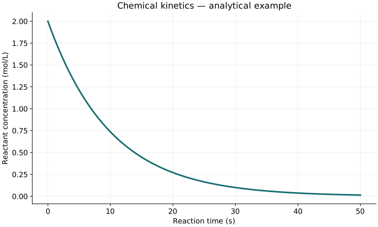
↑ Return to definitions and contentsGraphical worked example
Twenty worked examples
Open a problem to see its defined inputs, assumptions, equation, numerical substitution, result, and interpretation. Values are illustrative analytical exercises.
Example 01. First-order initial rate
Definitions & inputs. k=.2 s⁻¹,cA=3 mol/L.
Choose the governing model and isolate the requested quantity.
Insert the stated inputs in consistent units or the explicitly defined normalized units.
Evaluate the expression; the result uses the units shown.
Interpretation. The consumption coefficient is defined for A directly.
↑ Return to definitions and contentsExample 02. First-order concentration
Definitions & inputs. c0=2 mol/L,k=.1 s⁻¹,t=10 s.
Choose the governing model and isolate the requested quantity.
Insert the stated inputs in consistent units or the explicitly defined normalized units.
Evaluate the expression; the result uses the units shown.
Interpretation. Isothermal constant-volume conditions keep k constant.
↑ Return to definitions and contentsExample 03. First-order half-life
Definitions & inputs. k=.1 s⁻¹.
Choose the governing model and isolate the requested quantity.
Insert the stated inputs in consistent units or the explicitly defined normalized units.
Evaluate the expression; the result uses the units shown.
Interpretation. It does not depend on starting concentration.
↑ Return to definitions and contentsExample 04. Time to 90% conversion
Definitions & inputs. First-order k=.2 s⁻¹.
Choose the governing model and isolate the requested quantity.
Insert the stated inputs in consistent units or the explicitly defined normalized units.
Evaluate the expression; the result uses the units shown.
Interpretation. Conversion X is a fraction, not a percentage in the equation.
↑ Return to definitions and contentsExample 05. Measured first-order constant
Definitions & inputs. Concentration drops from 1 to .4 mol/L in 5 s.
Choose the governing model and isolate the requested quantity.
Insert the stated inputs in consistent units or the explicitly defined normalized units.
Evaluate the expression; the result uses the units shown.
Interpretation. More measurements are needed to establish first-order behavior.
↑ Return to definitions and contentsExample 06. Zero-order concentration
Definitions & inputs. c0=1 mol/L,k=.02 mol/(L s),t=20 s.
Choose the governing model and isolate the requested quantity.
Insert the stated inputs in consistent units or the explicitly defined normalized units.
Evaluate the expression; the result uses the units shown.
Interpretation. The law cannot continue into negative concentration.
↑ Return to definitions and contentsExample 07. Zero-order depletion time
Definitions & inputs. c0=1 mol/L,k=.02 mol/(L s).
Choose the governing model and isolate the requested quantity.
Insert the stated inputs in consistent units or the explicitly defined normalized units.
Evaluate the expression; the result uses the units shown.
Interpretation. Real kinetics may change as reactant becomes scarce.
↑ Return to definitions and contentsExample 08. Second-order concentration
Definitions & inputs. −dc/dt=kc²,k=.5 L/(mol s),c0=1 mol/L,t=2 s.
Choose the governing model and isolate the requested quantity.
Insert the stated inputs in consistent units or the explicitly defined normalized units.
Evaluate the expression; the result uses the units shown.
Interpretation. k is the species-consumption coefficient as explicitly defined.
↑ Return to definitions and contentsExample 09. Second-order half-life
Definitions & inputs. k=.5 L/(mol s),c0=2 mol/L.
Choose the governing model and isolate the requested quantity.
Insert the stated inputs in consistent units or the explicitly defined normalized units.
Evaluate the expression; the result uses the units shown.
Interpretation. Doubling c0 halves the half-life.
↑ Return to definitions and contentsExample 10. Rate change on doubling concentration
Definitions & inputs. Empirical order m=2.
Choose the governing model and isolate the requested quantity.
Insert the stated inputs in consistent units or the explicitly defined normalized units.
Evaluate the expression; the result uses the units shown.
Interpretation. A reaction’s written stoichiometry alone does not prove this order.
↑ Return to definitions and contentsExample 11. Arrhenius rate ratio
Definitions & inputs. Ea=50 kJ/mol,T1=300 K,T2=320 K,R=8.314462618.
Choose the governing model and isolate the requested quantity.
Insert the stated inputs in consistent units or the explicitly defined normalized units.
Evaluate the expression; the result uses the units shown.
Interpretation. The prefactor and mechanism are assumed unchanged.
↑ Return to definitions and contentsExample 12. Activation energy estimate
Definitions & inputs. Rate doubles from 300 to 310 K.
Choose the governing model and isolate the requested quantity.
Insert the stated inputs in consistent units or the explicitly defined normalized units.
Evaluate the expression; the result uses the units shown.
Interpretation. Two points estimate an apparent activation energy, not a unique mechanism.
↑ Return to definitions and contentsExample 13. Pseudo-first-order constant
Definitions & inputs. B maintained at .1 mol/L,k2=2 L/(mol s),r=k2 cA cB.
Choose the governing model and isolate the requested quantity.
Insert the stated inputs in consistent units or the explicitly defined normalized units.
Evaluate the expression; the result uses the units shown.
Interpretation. B must remain effectively constant throughout the experiment.
↑ Return to definitions and contentsExample 14. Parallel-path branch yield
Definitions & inputs. A→P k1=.3 s⁻¹,A→Q k2=.1 s⁻¹.
Choose the governing model and isolate the requested quantity.
Insert the stated inputs in consistent units or the explicitly defined normalized units.
Evaluate the expression; the result uses the units shown.
Interpretation. This is the final fraction through P for irreversible first-order branches.
↑ Return to definitions and contentsExample 15. Parallel-path remaining fraction
Definitions & inputs. k1=.3,k2=.1 s⁻¹,t=5 s.
Choose the governing model and isolate the requested quantity.
Insert the stated inputs in consistent units or the explicitly defined normalized units.
Evaluate the expression; the result uses the units shown.
Interpretation. Product concentrations require integrating each branch.
↑ Return to definitions and contentsExample 16. Reversible equilibrium fraction
Definitions & inputs. A⇌B first-order kf=.3,kr=.1 s⁻¹,total concentration 1 mol/L.
Choose the governing model and isolate the requested quantity.
Insert the stated inputs in consistent units or the explicitly defined normalized units.
Evaluate the expression; the result uses the units shown.
Interpretation. At equilibrium forward and reverse rates are equal, not zero.
↑ Return to definitions and contentsExample 17. Reversible relaxation time
Definitions & inputs. kf=.3,kr=.1 s⁻¹.
Choose the governing model and isolate the requested quantity.
Insert the stated inputs in consistent units or the explicitly defined normalized units.
Evaluate the expression; the result uses the units shown.
Interpretation. Deviations from the two-state equilibrium decay with this time constant.
↑ Return to definitions and contentsExample 18. Reactor residence time
Definitions & inputs. Volume 10 L,flow .5 L/s.
Choose the governing model and isolate the requested quantity.
Insert the stated inputs in consistent units or the explicitly defined normalized units.
Evaluate the expression; the result uses the units shown.
Interpretation. This is mean hydraulic residence time, not an identical path time in a stirred tank.
↑ Return to definitions and contentsExample 19. CSTR conversion
Definitions & inputs. First-order k=.1 s⁻¹,τ=20 s.
Choose the governing model and isolate the requested quantity.
Insert the stated inputs in consistent units or the explicitly defined normalized units.
Evaluate the expression; the result uses the units shown.
Interpretation. A perfectly mixed steady reactor has outlet concentration equal to tank concentration.
↑ Return to definitions and contentsExample 20. Plug-flow conversion
Definitions & inputs. First-order k=.1 s⁻¹,τ=20 s.
Choose the governing model and isolate the requested quantity.
Insert the stated inputs in consistent units or the explicitly defined normalized units.
Evaluate the expression; the result uses the units shown.
Interpretation. Ideal plug flow gives higher conversion here at the same kτ.
↑ Return to definitions and contentsSymbols and units
Each derivation and problem defines its own symbols and inputs. Symbols may be reused with different meanings in other subjects. Keep units consistent, retain sufficient precision during calculation, and apply the stated validity limits.