PHYSICS / ENGINEERING / COMPUTING
Electrical engineering models
From charge and circuit conservation to AC power, filters, transformers, and energy: four derivation pathways and twenty solved examples.
Matter pathway: atom → solid → liquid → gas → plasma. Quantum mechanics and quantum field theory provide foundations across the pathway; they are not additional phases. This is a connected modeling route, not a universal heating curve. Actual phases depend on pressure, composition, and kinetics.
1. Circuit conservation
Definitions & inputs. q charge, i current, v voltage, R resistance; signed currents enter a node.
Define flow of charge and the linear resistor law.
Apply charge conservation and loop energy conservation.
Equal series current adds drops; equal parallel voltage adds currents.
Interpretation. Reference directions determine signs; negative results indicate opposite flow.
↑ Return to definitions and contents2. Storage and transients
Definitions & inputs. C capacitance, L inductance, t time; Vs constant step source.
Constitutive relations connect storage to voltage/current.
Substitute resistor current into the node equation.
Integrate the first-order equation; integrate v dq for stored energy.
Interpretation. An inductor instead stores Li²/2; initial conditions determine transients.
↑ Return to definitions and contents3. Sinusoidal power
Definitions & inputs. j²=−1, ω angular frequency, RMS voltage V and current I, φ voltage-current phase.
Differentiate sinusoids using complex amplitudes.
Average instantaneous power to separate real and reactive terms.
The complex-power magnitude is apparent power in VA.
Interpretation. Power factor is cosφ only for sinusoidal waveforms without distortion.
↑ Return to definitions and contents4. Filters and conversion
Definitions & inputs. H voltage transfer, f frequency, N turns, subscripts p and s primary and secondary.
Apply a capacitive impedance divider.
Half-power cutoff follows |H|²=1/2; equal flux per turn sets voltage ratio.
Add three equal phase real powers and convert to line quantities.
Interpretation. Loading, winding loss, saturation, and harmonics require richer models.
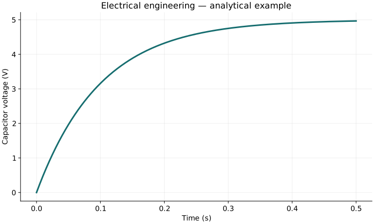
↑ Return to definitions and contentsGraphical worked example
Twenty worked examples
Open a problem to see its defined inputs, assumptions, equation, numerical substitution, result, and interpretation. Values are illustrative analytical exercises.
Example 01. Ohm-law current
Definitions & inputs. V=12 V, R=6 Ω.
Choose the governing model and isolate the requested quantity.
Insert the stated inputs in consistent units or the explicitly defined normalized units.
Evaluate the expression; the result uses the units shown.
Interpretation. Current follows the stated voltage polarity.
↑ Return to definitions and contentsExample 02. Resistor dissipation
Definitions & inputs. I=2 A, R=6 Ω.
Choose the governing model and isolate the requested quantity.
Insert the stated inputs in consistent units or the explicitly defined normalized units.
Evaluate the expression; the result uses the units shown.
Interpretation. This heat load must be compared with the resistor rating.
↑ Return to definitions and contentsExample 03. Series resistance
Definitions & inputs. R1=100 Ω, R2=220 Ω.
Choose the governing model and isolate the requested quantity.
Insert the stated inputs in consistent units or the explicitly defined normalized units.
Evaluate the expression; the result uses the units shown.
Interpretation. Both resistors carry the same current.
↑ Return to definitions and contentsExample 04. Parallel resistance
Definitions & inputs. R1=100 Ω, R2=300 Ω.
Choose the governing model and isolate the requested quantity.
Insert the stated inputs in consistent units or the explicitly defined normalized units.
Evaluate the expression; the result uses the units shown.
Interpretation. Equivalent resistance is less than either branch.
↑ Return to definitions and contentsExample 05. Unloaded divider
Definitions & inputs. Vin=10 V; upper R1=1 kΩ, lower R2=4 kΩ.
Choose the governing model and isolate the requested quantity.
Insert the stated inputs in consistent units or the explicitly defined normalized units.
Evaluate the expression; the result uses the units shown.
Interpretation. A connected load changes the lower effective resistance.
↑ Return to definitions and contentsExample 06. Node balance
Definitions & inputs. Currents entering are 3 A and 2 A; one current leaves.
Choose the governing model and isolate the requested quantity.
Insert the stated inputs in consistent units or the explicitly defined normalized units.
Evaluate the expression; the result uses the units shown.
Interpretation. This assumes no net charge accumulation at the node.
↑ Return to definitions and contentsExample 07. Capacitor charge
Definitions & inputs. C=100 μF, V=5 V.
Choose the governing model and isolate the requested quantity.
Insert the stated inputs in consistent units or the explicitly defined normalized units.
Evaluate the expression; the result uses the units shown.
Interpretation. Stored charge magnitude is equal on the two plates.
↑ Return to definitions and contentsExample 08. Capacitor energy
Definitions & inputs. C=100 μF, V=5 V.
Choose the governing model and isolate the requested quantity.
Insert the stated inputs in consistent units or the explicitly defined normalized units.
Evaluate the expression; the result uses the units shown.
Interpretation. Charging losses depend on the source circuit.
↑ Return to definitions and contentsExample 09. Inductor energy
Definitions & inputs. L=20 mH, I=2 A.
Choose the governing model and isolate the requested quantity.
Insert the stated inputs in consistent units or the explicitly defined normalized units.
Evaluate the expression; the result uses the units shown.
Interpretation. Use a nonsaturating linear inductance.
↑ Return to definitions and contentsExample 10. RC time constant
Definitions & inputs. R=10 kΩ, C=10 μF.
Choose the governing model and isolate the requested quantity.
Insert the stated inputs in consistent units or the explicitly defined normalized units.
Evaluate the expression; the result uses the units shown.
Interpretation. About 63.2% of a step is reached after one time constant.
↑ Return to definitions and contentsExample 11. RC charging at one time constant
Definitions & inputs. Vs=5 V, initially zero, t=τ.
Choose the governing model and isolate the requested quantity.
Insert the stated inputs in consistent units or the explicitly defined normalized units.
Evaluate the expression; the result uses the units shown.
Interpretation. The final voltage is 5 V only for negligible leakage and loading.
↑ Return to definitions and contentsExample 12. RC cutoff
Definitions & inputs. R=1 kΩ, C=100 nF.
Choose the governing model and isolate the requested quantity.
Insert the stated inputs in consistent units or the explicitly defined normalized units.
Evaluate the expression; the result uses the units shown.
Interpretation. The output amplitude is 1/√2 at cutoff.
↑ Return to definitions and contentsExample 13. Inductive reactance
Definitions & inputs. f=50 Hz, L=0.1 H.
Choose the governing model and isolate the requested quantity.
Insert the stated inputs in consistent units or the explicitly defined normalized units.
Evaluate the expression; the result uses the units shown.
Interpretation. Inductive voltage leads current by 90°.
↑ Return to definitions and contentsExample 14. Capacitive reactance magnitude
Definitions & inputs. f=50 Hz, C=100 μF.
Choose the governing model and isolate the requested quantity.
Insert the stated inputs in consistent units or the explicitly defined normalized units.
Evaluate the expression; the result uses the units shown.
Interpretation. Capacitive impedance has a negative imaginary part.
↑ Return to definitions and contentsExample 15. Series R-L impedance magnitude
Definitions & inputs. R=30 Ω, XL=40 Ω.
Choose the governing model and isolate the requested quantity.
Insert the stated inputs in consistent units or the explicitly defined normalized units.
Evaluate the expression; the result uses the units shown.
Interpretation. A 100 V RMS source would deliver 2 A RMS.
↑ Return to definitions and contentsExample 16. Single-phase real power
Definitions & inputs. V=230 V RMS, I=10 A RMS, power factor 0.8.
Choose the governing model and isolate the requested quantity.
Insert the stated inputs in consistent units or the explicitly defined normalized units.
Evaluate the expression; the result uses the units shown.
Interpretation. Apparent power is 2300 VA.
↑ Return to definitions and contentsExample 17. Ideal transformer output
Definitions & inputs. Vp=120 V RMS, Np=1000, Ns=100 turns.
Choose the governing model and isolate the requested quantity.
Insert the stated inputs in consistent units or the explicitly defined normalized units.
Evaluate the expression; the result uses the units shown.
Interpretation. Loaded regulation and winding losses are neglected.
↑ Return to definitions and contentsExample 18. Balanced three-phase power
Definitions & inputs. Line voltage 400 V RMS, line current 10 A RMS, power factor 0.9.
Choose the governing model and isolate the requested quantity.
Insert the stated inputs in consistent units or the explicitly defined normalized units.
Evaluate the expression; the result uses the units shown.
Interpretation. Line voltage differs from phase voltage in a star connection.
↑ Return to definitions and contentsExample 19. LC resonance
Definitions & inputs. L=10 mH, C=1 μF.
Choose the governing model and isolate the requested quantity.
Insert the stated inputs in consistent units or the explicitly defined normalized units.
Evaluate the expression; the result uses the units shown.
Interpretation. Resistance sets resonance width and amplitude.
↑ Return to definitions and contentsExample 20. Battery ideal energy
Definitions & inputs. Nominal voltage 12 V, capacity 10 Ah.
Choose the governing model and isolate the requested quantity.
Insert the stated inputs in consistent units or the explicitly defined normalized units.
Evaluate the expression; the result uses the units shown.
Interpretation. Usable energy depends on discharge rate, temperature, and cutoff.
↑ Return to definitions and contentsSymbols and units
Each derivation and problem defines its own symbols and inputs. Symbols may be reused with different meanings in other subjects. Keep units consistent, retain sufficient precision during calculation, and apply the stated validity limits.