Quantum mechanics: atoms to matter

1. States, probabilities, and the Schrödinger equation

Definitions & inputs. ψ is a normalized wavefunction; m is mass; V is potential energy; ℏ=h/(2π); H is the Hamiltonian. An observable is represented by a self-adjoint operator A.

1. Normalize the state. The squared amplitude is a probability density, so its units in three dimensions are inverse volume.

   $$\int |\psi(\mathbf r,t)|^2d^3r=1,\quad P(\Omega)=\int_\Omega|\psi|^2d^3r$$

2. The Schrödinger equation is a dynamical postulate here, not a consequence of Newton’s law.

   $$i\hbar\partial_t\psi=\hat H\psi,\quad\hat H=-\frac{\hbar^2}{2m}\nabla^2+V$$

3. For a time-independent Hamiltonian, separate the time phase to obtain the stationary eigenvalue problem.

   $$\psi=\phi e^{-iEt/\hbar}\quad\Rightarrow\quad\hat H\phi=E\phi$$

4. Expectation values and fluctuations describe repeated preparations. A stationary energy eigenstate need not have a definite position.

   $$\langle A\rangle=\int\psi^*\hat A\psi\,d^3r,\quad[\hat x,\hat p_x]=i\hbar,\quad\Delta x\Delta p_x\geq\hbar/2$$

Interpretation. Atomic binding, electronic bands, and quantum scattering use this same state-and-Hamiltonian framework.

• Tong — Quantum Mechanics: states, operators, and confinement ↗

2. Worked example: an electron in a one-nanometre box

Definitions & inputs. L=1.00 nm is the width; me=9.1093837×10⁻³¹ kg; ℏ=1.054571817×10⁻³⁴ J s; 1 eV=1.602176634×10⁻¹⁹ J. j=1,2,… labels levels.

1. Inside the box V=0. Impose zero amplitude at the impenetrable walls.

   $$-\frac{\hbar^2}{2m_e}\phi^{\prime\prime}=E\phi,\quad\phi(0)=\phi(L)=0$$

2. The left boundary removes the cosine; the right boundary discretizes the wave number.

   $$\phi=A\sin kx+B\cos kx,\quad B=0,\quad kL=j\pi$$

3. Normalize each eigenstate; the density is not uniform even though the potential is.

   $$1=A^2\int_0^L\sin^2(j\pi x/L)dx=A^2L/2,\quad\phi_j=\sqrt{2/L}\sin(j\pi x/L)$$

4. Insert the SI inputs and convert joules to electronvolts.

   $$E_j=\frac{\hbar^2\pi^2j^2}{2m_eL^2},\quad E_1=0.37603\ {\rm eV},\quad E_2=1.50412\ {\rm eV}$$

5. This is the photon wavelength matching the level separation; transition probability additionally depends on the coupling and selection rules.

   $$E_2-E_1=1.12809\ {\rm eV},\quad\lambda_\gamma=\frac{hc}{E_2-E_1}\simeq1099.1\ {\rm nm}$$

Interpretation. Reducing L raises the energies as 1/L². The plot below shows the dimensionless densities L|φj|², each integrating to one over x/L.

• Tong — Quantum Mechanics: states, operators, and confinement ↗

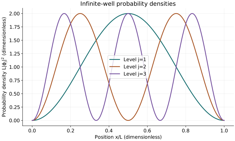
3. From the Coulomb potential to a bound atom

Definitions & inputs. For hydrogen, μ is the electron–proton reduced mass, e is the elementary charge, ε0 is vacuum permittivity, aμ is the reduced-mass Bohr radius, and j is the principal quantum number.

1. Separate the centre-of-mass motion and try a spherically symmetric decaying bound state.

   $$\hat H=-\frac{\hbar^2}{2\mu}\nabla^2-\frac{e^2}{4\pi\epsilon_0 r},\quad\psi_{1s}=A e^{-r/a}$$

2. Apply the radial Laplacian r⁻²∂r(r²∂r) to the trial state.

   $$\nabla^2e^{-r/a}=\left(\frac1{a^2}-\frac2{ar}\right)e^{-r/a}$$

3. For an eigenstate the right-hand side must be independent of r; set the coefficient of 1/r to zero.

   $$\frac{\hat H\psi}{\psi}=-\frac{\hbar^2}{2\mu a^2}+\frac1r\left(\frac{\hbar^2}{\mu a}-\frac{e^2}{4\pi\epsilon_0}\right)$$

4. This fixes the decay length and ground-state energy; radial normalization fixes A.

   $$a_\mu=\frac{4\pi\epsilon_0\hbar^2}{\mu e^2},\quad E_1=-\frac{\hbar^2}{2\mu a_\mu^2},\quad A=(\pi a_\mu^3)^{-1/2}$$

5. Solving the remaining angular and radial eigenproblems yields the full Coulomb spectrum; that general solution is quoted, not derived by the ground-state ansatz.

   $$E_j=-\frac{\mu e^4}{2(4\pi\epsilon_0)^2\hbar^2j^2}\simeq-\frac{13.6\ {\rm eV}}{j^2}$$

Interpretation. Atoms contain quantized bound electronic states. As atoms approach, their orbitals interact; the many-electron Hamiltonian, exchange, and screening determine bonds and bands.

• Tong — Quantum Mechanics: the hydrogen atom ↗

4. Worked example: hydrogen emission and an ionization threshold

Definitions & inputs. Use the rounded hydrogen scale 13.6 eV and hc=1239.841984 eV nm. Eγ is a photon energy; λγ its vacuum wavelength.

1. Evaluate the initial j=3 and final j=2 levels.

   $$E_2=-13.6/4=-3.40\ {\rm eV},\quad E_3=-13.6/9=-1.51111\ {\rm eV}$$

2. Energy conservation gives the Balmer-alpha scale; it is not a precision wavelength prediction.

   $$E_\gamma=E_3-E_2=1.88889\ {\rm eV},\quad\lambda_\gamma=1239.841984/1.88889\simeq656\ {\rm nm}$$

3. A photon at the ground-state ionization threshold leaves zero excess electron kinetic energy in this idealized energy accounting.

   $$E_{\rm ion,1}=0-E_1=13.6\ {\rm eV},\quad\lambda_{\rm threshold}=1239.841984/13.6\simeq91.2\ {\rm nm}$$

4. For a 20 eV absorbed photon, neglecting recoil leaves 6.40 eV for the electron. A real ionization rate also requires a cross section and photon flux.

   $$K_e\simeq E_\gamma-E_{\rm ion,1}=20.0-13.6=6.40\ {\rm eV}$$

Interpretation. Atomic energy scales enter gas spectra and ionization models. A threshold alone does not establish ionization equilibrium or collective plasma behavior.

• Tong — Quantum Mechanics: the hydrogen atom ↗
• PlasmaPy — Saha ionization relation ↗

5. Atom → solid: electronic energy surfaces and bands

Definitions & inputs. R denotes nuclear positions, r electronic coordinates, Tn nuclear kinetic energy, He the fixed-nuclei electronic Hamiltonian including nuclear repulsion, and Ua(R) an electronic energy surface.

1. First solve or approximate the electronic problem for fixed nuclei. Electron exchange and electron–electron interactions remain part of that problem.

   $$\hat H=\hat T_n+\hat H_e(\mathbf R),\quad\hat H_e(\mathbf R)\Phi_a(\mathbf r;\mathbf R)=U_a(\mathbf R)\Phi_a$$

2. Project onto a single electronic surface and neglect derivative couplings. Ua becomes an effective potential for nuclear motion.

   $$\Psi(\mathbf r,\mathbf R)\simeq\Phi_a(\mathbf r;\mathbf R)\chi(\mathbf R),\quad[\hat T_n+U_a(\mathbf R)]\chi\simeq E\chi$$

3. Near a stable configuration, first derivatives vanish and the quadratic expansion gives force constants and phonons. Anharmonic terms matter near melting.

   $$U_a(\mathbf R_0+\mathbf u)\simeq U_0+\frac12\sum_{I J}u_I K_{I J}u_J$$

4. A periodic effective one-electron potential permits Bloch states; u has lattice periodicity. Allowed energies form bands rather than isolated atomic levels.

   $$V(\mathbf r+\mathbf R_\ell)=V(\mathbf r),\quad\psi_{n\mathbf k}=e^{i\mathbf k\cdot\mathbf r}u_{n\mathbf k}(\mathbf r)$$

Interpretation. Electronic structure supplies the material-specific interactions used by solid, liquid, and gas models. Melting still requires free-energy comparison; it is not a change in the fundamental quantum laws.

• Tong — Electrons in Solids ↗
• Tong — Applications of Quantum Mechanics: atoms, bands, and phonons ↗

6. Worked example: a one-dimensional tight-binding band

Definitions & inputs. |j⟩ is an orthonormal orbital on site j, a is lattice spacing, εa its on-site energy, and t>0 is nearest-neighbor hopping. Choose εa=0 and t=1 eV.

1. Couple orbitals on adjacent atoms; the minus sign fixes the energy convention.

   $$\hat H=\epsilon_a\sum_j|j\rangle\langle j|-t\sum_j(|j\rangle\langle j+1|+|j+1\rangle\langle j|)$$

2. Apply H to a Bloch superposition and collect the two neighbor phase factors.

   $$|k\rangle=N^{-1/2}\sum_j e^{ikja}|j\rangle,\quad E(k)=\epsilon_a-t(e^{ika}+e^{-ika})$$

3. The bandwidth is 4t=4 eV. The plot uses ka/π from −1 to 1.

   $$E(k)=\epsilon_a-2t\cos ka,\quad E(0)=-2\ {\rm eV},\quad E(\pi/a)=2\ {\rm eV}$$

4. Expand cos(ka) near k=0 and match ℏ²k²/(2m*). The effective mass describes curvature near the band minimum.

   $$E(k)\simeq\epsilon_a-2t+ta^2k^2,\quad m^*=\frac{\hbar^2}{2ta^2}$$

Interpretation. Many coupled atomic orbitals produce a band. Filling, spin, interactions, and dimensionality determine whether this model can describe a conductor or insulator.

• Tong — Electrons in Solids ↗

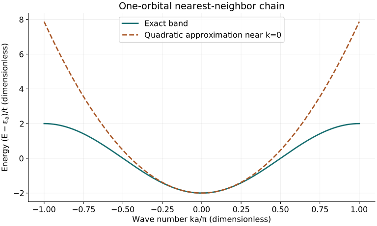
7. Quantum statistics → solid, liquid, gas, and plasma models

Definitions & inputs. β=1/(kBT), μ is chemical potential, ε is a single-particle energy, and λT=h/√(2πmkBT) is the thermal de Broglie wavelength. n is number density; gs counts internal spin states.

1. Bosons can share a state; fermionic occupation per state is at most one. These statistics apply to particles and suitable excitations in every phase.

   $$\bar n_{\rm B}(\epsilon)=\frac1{e^{\beta(\epsilon-\mu)}-1},\quad\bar n_{\rm F}(\epsilon)=\frac1{e^{\beta(\epsilon-\mu)}+1}$$

2. When state occupancy is small, both distributions approach Maxwell–Boltzmann statistics.

   $$e^{\beta(\epsilon-\mu)}\gg1\quad\Rightarrow\quad\bar n\simeq e^{-\beta(\epsilon-\mu)},\quad n\lambda_T^3/g_s\ll1$$

3. Classical nuclear motion additionally needs small quantum delocalization on relevant potential length scales and appropriate mode temperatures. Electrons may remain fully quantum.

   $$\hat H_n\longrightarrow H_{\rm cl}=\sum_I\frac{P_I^2}{2M_I}+U_a(\mathbf R)$$

4. A solid expansion, liquid configurational statistics, and gas collision descriptions approximate different regimes of the same underlying interactions.

   $$\text{solid: }U_a\simeq U_0+\tfrac12uKu;\quad\text{liquid/gas: sample }e^{-\beta U_a}$$

Interpretation. A liquid can be quantum (for example superfluid helium), and plasma electrons can be degenerate. Phase labels alone do not justify a classical approximation.

• Tong — Statistical Physics: quantum gases ↗
• Tong — Kinetic Theory: Liouville, BBGKY, Boltzmann and fluid equations ↗

8. Worked example: test the classical-gas approximation

Definitions & inputs. Use T=300 K. For helium atoms use m=6.64648×10⁻²⁷ kg, n=2.45×10²⁵ m⁻³, gs=1. Separately use electrons at n=10²⁹ m⁻³, me=9.1093837×10⁻³¹ kg, gs=2.

1. Calculate helium’s thermal wavelength in SI units.

   $$\lambda_{T,\rm He}=\frac{6.62607015\times10^{-34}}{\sqrt{2\pi(6.64648\times10^{-27})(1.380649\times10^{-23})(300)}}\simeq0.0504\ {\rm nm}$$

2. Exchange degeneracy is negligible for these helium inputs; interactions must still be checked separately.

   $$n\lambda_{T,\rm He}^3\simeq3.14\times10^{-6}\ll1$$

3. At the chosen electron density, classical Maxwell–Boltzmann statistics fail strongly.

   $$\lambda_{T,e}\simeq4.30\ {\rm nm},\quad n\lambda_{T,e}^3/2\simeq3.98\times10^3\gg1$$

4. The ideal spin-half electron gas has T≪TF and is degenerate; use Fermi statistics. This free-gas Fermi energy is not a material-specific band calculation.

   $$E_F=\frac{\hbar^2}{2m_e}(3\pi^2n)^{2/3}\simeq7.86\ {\rm eV},\quad T_F=E_F/k_B\simeq9.12\times10^4\ {\rm K}$$

Interpretation. Heavy atoms may move classically while electrons in the same broad temperature range require quantum statistics.

• Tong — Statistical Physics: quantum gases ↗

How the quantum foundations connect to each state

Read the atom-to-plasma route below as a sequence of modeling choices. Cooling, heating, compression, and chemical changes can follow different physical paths.

Related models in the main catalog

• Schrödinger model — equation, applications, and worked graphs
• Quantum harmonic oscillator — equation, applications, and worked graphs
• Tight-binding model — equation, applications, and worked graphs
• Dirac model — equation, applications, and worked graphs

Return to Modeling · Numerical ModelingSensorsMathematics

Typical sensors and experimental connections

Spectrometer sensor · Single-photon avalanche diode (SPAD) · Interferometric displacement sensor

These are examples of instruments used to measure relevant observables, calibrate parameters, or test a physical system. They do not directly measure every abstract model quantity or prove a theory by themselves. Choose bandwidth, range, environment and uncertainty for the actual experiment.

Explore the dedicated Sensors site →

Mathematical tools and foundations

Eigenvalues and normal modes · Complex exponentials and phasors

Use the stated mathematical conditions together with the physical assumptions. Explore the Mathematics atlas →