PHYSICS / ENGINEERING / COMPUTING
Continuum mechanics: motion, stress and conservation
Build the common language of solid and fluid models from deformation maps through conservation laws and constitutive closure.
Matter pathway: atom → solid → liquid → gas → plasma. Quantum mechanics and quantum field theory provide foundations across the pathway; they are not additional phases. This is a connected modeling route, not a universal heating curve. Actual phases depend on pressure, composition, and kinetics.
1. Motion and finite deformation
Definitions & inputs. X reference position,x current position,F deformation gradient,J volume ratio.
Differentiate the motion with respect to the reference coordinates.
F changes material line elements and its determinant changes volumes.
Green strain measures squared length change and is invariant under superposed rigid rotation.
Interpretation. For small gradients use ε=sym∇u, but a finite rigid rotation must not create spurious strain.
↑ Return to definitions and contents2. Traction and stress measures
Definitions & inputs. σ Cauchy stress,n current unit normal,P first Piola stress,ρ density.
Cauchy traction maps a cut-plane normal into force per current area.
Transform current-area forces to reference-area forces using Nanson’s relation.
Linear momentum gives the stress divergence; angular momentum gives symmetry under the stated assumptions.
Interpretation. Keep reference and current configurations consistent when computing stress or boundary work.
↑ Return to definitions and contents3. Mass and internal energy
Definitions & inputs. e specific internal energy,q heat flux,r volumetric heat supply per mass,L velocity gradient,D=symL.
Material mass conservation gives both finite and differential statements.
Stress power, heat flow and heat generation change internal energy.
Fourier closure supplies a thermal constitutive law when local diffusion is appropriate.
Interpretation. Conservation equations alone do not select elasticity, viscosity or plasticity.
↑ Return to definitions and contents4. Constitutive closure and model hierarchy
Definitions & inputs. λ,G Lamé constants,K bulk modulus,μ dynamic viscosity.
Linear isotropic elasticity connects stress to strain.
Convert between common elastic coefficients.
In an incompressible Newtonian fluid stress depends on strain rate, with pressure enforcing incompressibility.
Interpretation. FEM often discretizes solid weak forms; finite volume methods enforce fluid conservation. Objectivity, positivity of dissipation and boundary conditions must accompany either choice.
↑ Return to definitions and contentsGraphical worked example
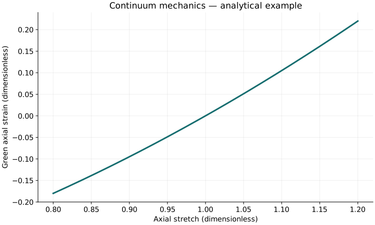
Twenty worked examples
Open a problem to see its defined inputs, assumptions, equation, numerical substitution, result, and interpretation. Values are illustrative analytical exercises.
Example 01. Axial stretch
Definitions & inputs. Length1m becomes1.02m.
Choose the governing model and isolate the requested quantity.
Insert the stated inputs in consistent units or the explicitly defined normalized units.
Evaluate the expression; the result uses the units shown.
Interpretation. Stretch is a ratio, not strain.
↑ Return to definitions and contentsExample 02. Engineering strain
Definitions & inputs. Samebar.
Choose the governing model and isolate the requested quantity.
Insert the stated inputs in consistent units or the explicitly defined normalized units.
Evaluate the expression; the result uses the units shown.
Interpretation. Small-strain measure.
↑ Return to definitions and contentsExample 03. Green axial strain
Definitions & inputs. Stretch1.02.
Choose the governing model and isolate the requested quantity.
Insert the stated inputs in consistent units or the explicitly defined normalized units.
Evaluate the expression; the result uses the units shown.
Interpretation. Finite-strain measure.
↑ Return to definitions and contentsExample 04. Logarithmic axial strain
Definitions & inputs. Stretch1.02.
Choose the governing model and isolate the requested quantity.
Insert the stated inputs in consistent units or the explicitly defined normalized units.
Evaluate the expression; the result uses the units shown.
Interpretation. Adds for sequential coaxial stretches.
↑ Return to definitions and contentsExample 05. Volume ratio
Definitions & inputs. F=diag(1.1,1,.9).
Choose the governing model and isolate the requested quantity.
Insert the stated inputs in consistent units or the explicitly defined normalized units.
Evaluate the expression; the result uses the units shown.
Interpretation. Positive determinant preserves orientation.
↑ Return to definitions and contentsExample 06. Density change
Definitions & inputs. ρ0=1000kg/m³,J=.99.
Choose the governing model and isolate the requested quantity.
Insert the stated inputs in consistent units or the explicitly defined normalized units.
Evaluate the expression; the result uses the units shown.
Interpretation. Material mass is conserved.
↑ Return to definitions and contentsExample 07. Rigid rotation strain
Definitions & inputs. F orthogonal.
Choose the governing model and isolate the requested quantity.
Insert the stated inputs in consistent units or the explicitly defined normalized units.
Evaluate the expression; the result uses the units shown.
Interpretation. Exact finite strain vanishes under rigid motion.
↑ Return to definitions and contentsExample 08. Normal traction
Definitions & inputs. σxx=20MPa,n=(1,0,0).
Choose the governing model and isolate the requested quantity.
Insert the stated inputs in consistent units or the explicitly defined normalized units.
Evaluate the expression; the result uses the units shown.
Interpretation. Shear traction may also exist if σyx orσzx is nonzero.
↑ Return to definitions and contentsExample 09. Pressure from stress
Definitions & inputs. Diagonal stresses−10,−20,−30MPa.
Choose the governing model and isolate the requested quantity.
Insert the stated inputs in consistent units or the explicitly defined normalized units.
Evaluate the expression; the result uses the units shown.
Interpretation. Pressure is positive in compression.
↑ Return to definitions and contentsExample 10. Deviatoric stress component
Definitions & inputs. Sameσxx=−10MPa,p20MPa.
Choose the governing model and isolate the requested quantity.
Insert the stated inputs in consistent units or the explicitly defined normalized units.
Evaluate the expression; the result uses the units shown.
Interpretation. Deviatoric stress has zero trace.
↑ Return to definitions and contentsExample 11. Shear modulus
Definitions & inputs. E200GPa,ν.3.
Choose the governing model and isolate the requested quantity.
Insert the stated inputs in consistent units or the explicitly defined normalized units.
Evaluate the expression; the result uses the units shown.
Interpretation. Isotropic stable linear elasticity.
↑ Return to definitions and contentsExample 12. Bulk modulus
Definitions & inputs. E200GPa,ν.3.
Choose the governing model and isolate the requested quantity.
Insert the stated inputs in consistent units or the explicitly defined normalized units.
Evaluate the expression; the result uses the units shown.
Interpretation. Incompressibility corresponds to largeK, not zeroK.
↑ Return to definitions and contentsExample 13. Uniaxial stress
Definitions & inputs. E200GPa,ε.001.
Choose the governing model and isolate the requested quantity.
Insert the stated inputs in consistent units or the explicitly defined normalized units.
Evaluate the expression; the result uses the units shown.
Interpretation. Uniaxial stress state with free lateral contraction.
↑ Return to definitions and contentsExample 14. Lateral strain
Definitions & inputs. ν.3,axialε.001.
Choose the governing model and isolate the requested quantity.
Insert the stated inputs in consistent units or the explicitly defined normalized units.
Evaluate the expression; the result uses the units shown.
Interpretation. Free lateral surfaces.
↑ Return to definitions and contentsExample 15. Hydrostatic volume strain
Definitions & inputs. p100MPa,K100GPa.
Choose the governing model and isolate the requested quantity.
Insert the stated inputs in consistent units or the explicitly defined normalized units.
Evaluate the expression; the result uses the units shown.
Interpretation. Linear compression estimate.
↑ Return to definitions and contentsExample 16. Viscous shear stress
Definitions & inputs. μ.001Pa·s,du/dy100/s.
Choose the governing model and isolate the requested quantity.
Insert the stated inputs in consistent units or the explicitly defined normalized units.
Evaluate the expression; the result uses the units shown.
Interpretation. Newtonian simple shear.
↑ Return to definitions and contentsExample 17. Heat flux
Definitions & inputs. k10W/(mK),dT/dx20K/m.
Choose the governing model and isolate the requested quantity.
Insert the stated inputs in consistent units or the explicitly defined normalized units.
Evaluate the expression; the result uses the units shown.
Interpretation. Negative sign denotes down-gradient flow.
↑ Return to definitions and contentsExample 18. Volumetric strain rate
Definitions & inputs. Velocity gradients .1,.2,−.1/s.
Choose the governing model and isolate the requested quantity.
Insert the stated inputs in consistent units or the explicitly defined normalized units.
Evaluate the expression; the result uses the units shown.
Interpretation. Positive divergence locally expands material.
↑ Return to definitions and contentsExample 19. Density time derivative
Definitions & inputs. ρ1000kg/m³,divv.2/s.
Choose the governing model and isolate the requested quantity.
Insert the stated inputs in consistent units or the explicitly defined normalized units.
Evaluate the expression; the result uses the units shown.
Interpretation. Material derivative, not fixed-point derivative.
↑ Return to definitions and contentsExample 20. Elastic energy density
Definitions & inputs. σ200MPa,ε.001.
Choose the governing model and isolate the requested quantity.
Insert the stated inputs in consistent units or the explicitly defined normalized units.
Evaluate the expression; the result uses the units shown.
Interpretation. Uniaxial proportional linear loading.
↑ Return to definitions and contentsSymbols and units
Each derivation and problem defines its own symbols and inputs. Symbols may be reused with different meanings in other subjects. Keep units consistent, retain sufficient precision during calculation, and apply the stated validity limits.