PHYSICS / ENGINEERING / COMPUTING
Particle physics models
Connect relativistic kinematics, particle reactions, decays, and counting experiments through definitions, derivations, and twenty worked examples.
Matter pathway: atom → solid → liquid → gas → plasma. Quantum mechanics and quantum field theory provide foundations across the pathway; they are not additional phases. This is a connected modeling route, not a universal heating curve. Actual phases depend on pressure, composition, and kinetics.
1. Four-momentum and invariant mass
Definitions & inputs. pμ=(E/c,p); m is rest mass; s is squared centre-of-mass energy when c=1.
Lorentz invariance fixes the mass shell.
Express energy and momentum in a chosen inertial frame.
Add four-momenta before taking the invariant; masses do not generally add.
Expand the incoming invariant for collider or fixed-target kinematics.
Interpretation. Kinematic accessibility does not imply a reaction has an appreciable cross section.
↑ Return to definitions and contents2. Two-body decay and lifetimes
Definitions & inputs. M is parent rest mass, m1,m2 daughter masses, Γ energy width, τ proper mean lifetime.
Use energy and momentum conservation in the parent rest frame.
Subtract daughter mass-shell equations and solve.
Integrate a constant decay probability per proper time.
Energy width sets proper lifetime; time dilation sets mean flight distance.
Interpretation. A mean decay length is not a deterministic stopping distance.
↑ Return to definitions and contents3. Cross sections and experimental counts
Definitions & inputs. σ is interaction cross section, luminosity ℒ is incident flux overlap per area per time, ε selection efficiency, B branching fraction.
Rate is luminosity times effective interaction area.
Include the desired decay channel and detection/selection losses.
Independent event counts follow a Poisson model.
Invert a background-subtracted counting model; propagate background and calibration uncertainties separately.
Interpretation. A counting estimate is not automatically a discovery significance.
↑ Return to definitions and contents4. Symmetries, interactions, and effective models
Definitions & inputs. ψ denotes fermion fields, Aμ gauge fields; g a coupling; Oi effective operators with scaling dimension di; Λ an energy cutoff.
Gauge interactions enter through covariant derivatives.
Higher-dimension interactions are suppressed at low energy under a controlled effective expansion.
Check scale separation before truncating an effective theory.
Interpretation. The Standard Model combines strong, weak, and electromagnetic interactions; gravity requires a separate framework here.
↑ Return to definitions and contentsGraphical worked example
Twenty worked examples
Open a problem to see its defined inputs, assumptions, equation, numerical substitution, result, and interpretation. Values are illustrative analytical exercises.
Example 01. Photon wavelength
Definitions & inputs. Photon energy E=1 MeV; hc=1.239841984 MeV pm.
Choose the governing model and isolate the requested quantity.
Insert the stated inputs in consistent units or the explicitly defined normalized units.
Evaluate the expression; the result uses the units shown.
Interpretation. Higher photon energy corresponds to shorter wavelength.
↑ Return to definitions and contentsExample 02. Lorentz factor at 0.8c
Definitions & inputs. β=v/c=0.8.
Choose the governing model and isolate the requested quantity.
Insert the stated inputs in consistent units or the explicitly defined normalized units.
Evaluate the expression; the result uses the units shown.
Interpretation. This factor multiplies rest energy and dilates mean lifetime.
↑ Return to definitions and contentsExample 03. Electron kinetic energy
Definitions & inputs. Electron mc²=0.511 MeV and γ=3.
Choose the governing model and isolate the requested quantity.
Insert the stated inputs in consistent units or the explicitly defined normalized units.
Evaluate the expression; the result uses the units shown.
Interpretation. Total energy includes rest energy; kinetic energy does not.
↑ Return to definitions and contentsExample 04. Momentum from total energy
Definitions & inputs. Particle E=5 GeV, mc²=3 GeV.
Choose the governing model and isolate the requested quantity.
Insert the stated inputs in consistent units or the explicitly defined normalized units.
Evaluate the expression; the result uses the units shown.
Interpretation. The momentum itself is 4 GeV/c.
↑ Return to definitions and contentsExample 05. Head-on photon invariant mass
Definitions & inputs. E1=2 GeV, E2=8 GeV, angle θ=π.
Choose the governing model and isolate the requested quantity.
Insert the stated inputs in consistent units or the explicitly defined normalized units.
Evaluate the expression; the result uses the units shown.
Interpretation. Opposite photon momenta can produce a nonzero system invariant mass.
↑ Return to definitions and contentsExample 06. Symmetric collider energy
Definitions & inputs. Two equal-mass beams have E=10 GeV each and opposite momenta.
Choose the governing model and isolate the requested quantity.
Insert the stated inputs in consistent units or the explicitly defined normalized units.
Evaluate the expression; the result uses the units shown.
Interpretation. Total momentum vanishes in the centre-of-mass frame.
↑ Return to definitions and contentsExample 07. Fixed-target centre-of-mass energy
Definitions & inputs. Projectile total E=10 GeV; projectile and stationary target mass energies m=1 GeV.
Choose the governing model and isolate the requested quantity.
Insert the stated inputs in consistent units or the explicitly defined normalized units.
Evaluate the expression; the result uses the units shown.
Interpretation. A fixed-target experiment has less centre-of-mass energy than equal head-on beam energies.
↑ Return to definitions and contentsExample 08. Two-photon decay
Definitions & inputs. Parent rest energy Mc²=0.135 GeV.
Choose the governing model and isolate the requested quantity.
Insert the stated inputs in consistent units or the explicitly defined normalized units.
Evaluate the expression; the result uses the units shown.
Interpretation. Both photons have equal and opposite momenta in this frame.
↑ Return to definitions and contentsExample 09. Massive two-body daughter energy
Definitions & inputs. M=5 GeV, m1=1 GeV, m2=2 GeV in c=1 units.
Choose the governing model and isolate the requested quantity.
Insert the stated inputs in consistent units or the explicitly defined normalized units.
Evaluate the expression; the result uses the units shown.
Interpretation. The other daughter carries 2.8 GeV, conserving energy.
↑ Return to definitions and contentsExample 10. Lifetime from a decay width
Definitions & inputs. Γ=1 keV=10⁻⁶ GeV; ℏ=6.582119569×10⁻²⁵ GeV s.
Choose the governing model and isolate the requested quantity.
Insert the stated inputs in consistent units or the explicitly defined normalized units.
Evaluate the expression; the result uses the units shown.
Interpretation. A broader width means a shorter proper lifetime.
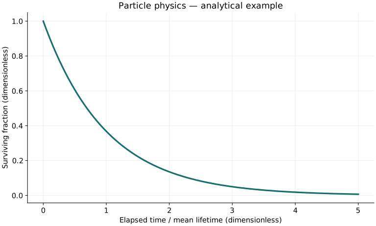
↑ Return to definitions and contentsExample 11. Survival after two lifetimes
Definitions & inputs. Elapsed proper time t=2τ.
Choose the governing model and isolate the requested quantity.
Insert the stated inputs in consistent units or the explicitly defined normalized units.
Evaluate the expression; the result uses the units shown.
Interpretation. About 13.5% survive.
↑ Return to definitions and contentsExample 12. Mean flight length
Definitions & inputs. βγ=10, proper τ=2.2 µs, c=299792458 m/s.
Choose the governing model and isolate the requested quantity.
Insert the stated inputs in consistent units or the explicitly defined normalized units.
Evaluate the expression; the result uses the units shown.
Interpretation. Individual decay locations follow a distribution.
↑ Return to definitions and contentsExample 13. Produced collision events
Definitions & inputs. Integrated luminosity 100 fb⁻¹; cross section 2 fb.
Choose the governing model and isolate the requested quantity.
Insert the stated inputs in consistent units or the explicitly defined normalized units.
Evaluate the expression; the result uses the units shown.
Interpretation. The inverse-area units cancel.
↑ Return to definitions and contentsExample 14. Selected decay yield
Definitions & inputs. Nproduced=1000; branching B=0.1; efficiency ε=0.6.
Choose the governing model and isolate the requested quantity.
Insert the stated inputs in consistent units or the explicitly defined normalized units.
Evaluate the expression; the result uses the units shown.
Interpretation. Branching and efficiency reduce expected yield separately.
↑ Return to definitions and contentsExample 15. Poisson relative precision
Definitions & inputs. Expected count μ=400.
Choose the governing model and isolate the requested quantity.
Insert the stated inputs in consistent units or the explicitly defined normalized units.
Evaluate the expression; the result uses the units shown.
Interpretation. The counting-only fractional uncertainty is 5%.
↑ Return to definitions and contentsExample 16. Cross section after subtraction
Definitions & inputs. Nobs=120, Nbg=20, luminosity 10 pb⁻¹, efficiency 0.5, B=1.
Choose the governing model and isolate the requested quantity.
Insert the stated inputs in consistent units or the explicitly defined normalized units.
Evaluate the expression; the result uses the units shown.
Interpretation. This point estimate needs uncertainty propagation for inference.
↑ Return to definitions and contentsExample 17. Momentum from track curvature
Definitions & inputs. Charge magnitude |q|=e, transverse field B=2 T, radius r=1 m.
Choose the governing model and isolate the requested quantity.
Insert the stated inputs in consistent units or the explicitly defined normalized units.
Evaluate the expression; the result uses the units shown.
Interpretation. The formula measures transverse momentum relative to the field.
↑ Return to definitions and contentsExample 18. Two-flavor oscillation probability
Definitions & inputs. sin²(2θ)=1; phase Δ=1.267Δm²[eV²]L[km]/E[GeV]=π/4.
Choose the governing model and isolate the requested quantity.
Insert the stated inputs in consistent units or the explicitly defined normalized units.
Evaluate the expression; the result uses the units shown.
Interpretation. The supplied phase produces 50% conversion in this model.
↑ Return to definitions and contentsExample 19. Momentum-resolution propagation
Definitions & inputs. pT∝Br; fractional B error 1%, radius error 2%, independent.
Choose the governing model and isolate the requested quantity.
Insert the stated inputs in consistent units or the explicitly defined normalized units.
Evaluate the expression; the result uses the units shown.
Interpretation. The combined fractional uncertainty is about 2.24%.
↑ Return to definitions and contentsExample 20. Effective-theory suppression
Definitions & inputs. Leading correction scales as (E/Λ)²; E=100 GeV, Λ=1000 GeV, coefficient one.
Choose the governing model and isolate the requested quantity.
Insert the stated inputs in consistent units or the explicitly defined normalized units.
Evaluate the expression; the result uses the units shown.
Interpretation. A one-percent power-counting estimate is not a computed cross-section correction.
↑ Return to definitions and contentsSymbols and units
Each derivation and problem defines its own symbols and inputs. Symbols may be reused with different meanings in other subjects. Keep units consistent, retain sufficient precision during calculation, and apply the stated validity limits.