Quantum field theory: fields to matter

1. From a classical field to its equation of motion

Definitions & inputs. φ(x,t) is a real scalar field, L is its Lagrangian density, and m is its mass parameter. In this section use natural units ℏ=c=1 and metric (+,−,−,−).

1. The action weights spacetime histories. The kinetic and mass terms specify the free scalar model.

   $$S=\int d^4x\,\mathcal L,\quad\mathcal L=\tfrac12\partial_\mu\phi\partial^\mu\phi-\tfrac12m^2\phi^2$$

2. Vary the action, integrate the derivative term by parts, and hold the boundary variation fixed at zero.

   $$\partial_\mu\frac{\partial\mathcal L}{\partial(\partial_\mu\phi)}-\frac{\partial\mathcal L}{\partial\phi}=0\quad\Rightarrow\quad(\partial_t^2-\nabla^2+m^2)\phi=0$$

3. Each Fourier component obeys a harmonic-oscillator equation with this frequency.

   $$\phi\propto e^{-i\omega t+i\mathbf k\cdot\mathbf x}\quad\Rightarrow\quad\omega_{\mathbf k}^2=|\mathbf k|^2+m^2$$

4. Restoring SI units gives the relativistic energy–momentum relation.

   $$E^2=p^2c^2+m^2c^4$$

Interpretation. A field supplies a continuum of coupled degrees of freedom. Fourier modes turn the free theory into independent oscillators.

• Tong — Quantum Field Theory: canonical quantization, spinors, and QED ↗

2. Quantize modes: particles and quasiparticles

Definitions & inputs. π=∂tφ is the canonical momentum field; ak and ak† lower and raise occupation of a mode. Use a finite periodic box and discrete modes to keep normalization explicit; ℏ is restored below.

1. Promote fields and momenta to operators with equal-time canonical commutators.

   $$[\hat\phi(\mathbf x),\hat\pi(\mathbf y)]=i\hbar\delta^3(\mathbf x-\mathbf y),\quad[\hat a_{\mathbf k},\hat a^\dagger_{\mathbf q}]=\delta_{\mathbf k\mathbf q}$$

2. The oscillator Hamiltonian counts excitation quanta plus a zero-point contribution.

   $$\hat H=\sum_{\mathbf k}\hbar\omega_{\mathbf k}(\hat a^\dagger_{\mathbf k}\hat a_{\mathbf k}+\tfrac12),\quad \hat N_{\mathbf k}=\hat a^\dagger_{\mathbf k}\hat a_{\mathbf k}$$

3. One creation operation adds a quantum of energy. A photon is a quantum of an electromagnetic mode; a phonon is a quantum of a lattice vibration.

   $$\hat a^\dagger|n\rangle=\sqrt{n+1}|n+1\rangle,\quad\Delta E=\hbar\omega$$

4. Sum a geometric series and its derivative to obtain the thermal bosonic occupation for modes of zero chemical potential.

   $$\bar n=\frac{\sum_{n=0}^\infty n e^{-\beta\hbar\omega n}}{\sum_{n=0}^\infty e^{-\beta\hbar\omega n}}=\frac1{e^{\beta\hbar\omega}-1}$$

Interpretation. Continuum vacuum-energy sums require regularization and a physical renormalization prescription; the formal sum is not a finite predicted absolute energy. QFT also describes low-energy collective excitations in matter.

• Tong — Quantum Field Theory: canonical quantization, spinors, and QED ↗
• Tong — Statistical Physics: quantum gases ↗

3. Worked example: a thermal phonon mode

Definitions & inputs. Take a harmonic mode with ℏω=20.0 meV at T=300 K, so kBT=25.8520 meV. nbar is its average excitation count.

1. Compare the mode energy with the thermal energy.

   $$x=\hbar\omega/(k_BT)=20.0/25.8520=0.773635$$

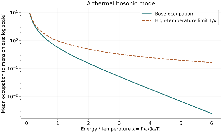
2. Use the Bose occupation, not a classical equipartition assumption.

   $$\bar n=1/(e^x-1)\simeq0.8564$$

3. Include the 10 meV zero-point energy of this oscillator.

   $$\bar E=\hbar\omega(\bar n+\tfrac12)\simeq27.13\ {\rm meV}$$

4. Differentiate the energy with respect to T at fixed ω. At high T this approaches kB; at low T it tends to zero.

   $$C=k_B\frac{x^2e^x}{(e^x-1)^2}\simeq0.9516\,k_B$$

Interpretation. The occupation graph compares the exact Bose result with its high-temperature limit nbar≈1/x. Quantized lattice modes connect the atomistic solid to thermal models.

• Tong — Statistical Physics: quantum gases ↗
• Phonopy — force constants, dynamical matrix and thermodynamics ↗

4. Nonrelativistic fields connect atoms, liquids, and quantum gases

Definitions & inputs. Ψhat(r) destroys a bosonic atom at r; m is atomic mass; Vext is an external trap. gB=4πℏ²as/m is the low-energy contact coupling and as is the s-wave scattering length. gB is not the liquid pair distribution g(r).

1. Write kinetic, external-potential, and two-body contact terms in field language. The factor one-half avoids double counting.

   $$\hat H=\int d^3r\left[\hat\Psi^\dagger\left(-\frac{\hbar^2\nabla^2}{2m}+V_{\rm ext}\right)\hat\Psi+\frac{g_B}{2}\hat\Psi^\dagger\hat\Psi^\dagger\hat\Psi\hat\Psi\right]$$

2. The Heisenberg equation evolves the operator field and contains interaction correlations.

   $$i\hbar\partial_t\hat\Psi=[\hat\Psi,\hat H]$$

3. Approximate the macroscopically occupied condensate by a classical complex field and factorize correlations: the Gross–Pitaevskii equation.

   $$\hat\Psi\longrightarrow\psi,\quad i\hbar\partial_t\psi=\left(-\frac{\hbar^2\nabla^2}{2m}+V_{\rm ext}+g_B|\psi|^2\right)\psi$$

4. A uniform stationary solution fixes the chemical potential at mean-field level.

   $$\psi_0=\sqrt n e^{-i\mu t/\hbar},\quad V_{\rm ext}=0\quad\Rightarrow\quad\mu=g_Bn$$

Interpretation. Second quantization is a language for many particles, not a second application of quantization to already quantum particles. Nonrelativistic field theories can conserve total atom number.

• Dalfovo et al. — Theory of Bose–Einstein condensation in trapped gases ↗

5. Worked example: derive a sound mode from a quantum field

Definitions & inputs. Perturb the uniform condensate: δψ=u exp[i(k·r−ωt)]+v* exp[−i(k·r−ωt)]. εk=ℏ²k²/(2m). Illustrative inputs m=1.44316×10⁻²⁵ kg, as=5.3 nm, n=10²⁰ m⁻³.

1. Insert the perturbed field into Gross–Pitaevskii, subtract the uniform solution, and retain terms linear in u and v.

   $$\hbar\omega\begin{pmatrix}u\\v\end{pmatrix}=\begin{pmatrix}\epsilon_k+g_Bn&g_Bn\\-g_Bn&-(\epsilon_k+g_Bn)\end{pmatrix}\begin{pmatrix}u\\v\end{pmatrix}$$

2. Set the determinant of the two-by-two eigenvalue problem to zero.

   $$(\hbar\omega)^2=(\epsilon_k+g_Bn)^2-(g_Bn)^2=\epsilon_k(\epsilon_k+2g_Bn)$$

3. At small k the excitation is sound; ξ is the healing length under the stated convention. At large k the leading term is the free-particle energy.

   $$\hbar\omega\simeq\hbar c_sk\ (k\to0),\quad c_s=\sqrt{g_Bn/m},\quad\xi=\hbar/\sqrt{2mg_Bn}$$

4. Check diluteness, then evaluate interaction energy, sound speed, and healing length.

   $$n a_s^3=1.49\times10^{-5},\quad g_Bn\simeq5.13\times10^{-31}\ {\rm J},\quad c_s\simeq1.89\ {\rm mm\,s^{-1}},\quad\xi\simeq0.274\ {\rm \mu m}$$

5. This dimensionless expression generates the plotted crossover from collective sound to particle-like motion.

   $$q=k\xi,\qquad\frac{\hbar\omega}{g_Bn}=\sqrt{q^2(q^2+2)}$$

Interpretation. A field model produces a macroscopic sound wave through controlled approximations. Different liquid regimes need different effective descriptions.

• Dalfovo et al. — Theory of Bose–Einstein condensation in trapped gases ↗

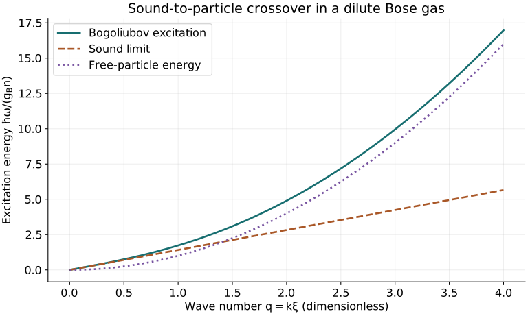
6. Electromagnetic quantum fields → atomic physics

Definitions & inputs. ψ is now a Dirac spinor, Aμ the electromagnetic potential, Fμν=∂μAν−∂νAμ, q the particle charge, and Dμ=∂μ+iqAμ. Natural units ℏ=c=1 are used only in the first equation.

1. Matter and electromagnetic fields interact through the covariant derivative. Fermionic and gauge quantization differ from the scalar example.

   $$\mathcal L_{\rm QED}=\bar\psi(i\gamma^\mu D_\mu-m)\psi-\tfrac14F_{\mu\nu}F^{\mu\nu}$$

2. Expand at p≪mc; remove the rest-energy phase to identify the nonrelativistic kinetic term.

   $$E=\sqrt{m^2c^4+p^2c^2}=mc^2+\frac{p^2}{2m}-\frac{p^4}{8m^3c^2}+\cdots$$

3. The low-energy spin-half theory includes spin coupling, with leading Dirac gyromagnetic factor two; further relativistic and radiative terms are omitted.

   $$\hat H_{\rm Pauli}\simeq\frac{(\hat{\mathbf p}-q\mathbf A)^2}{2m}+q\Phi-\frac{q\hbar}{2m}\boldsymbol\sigma\cdot\mathbf B$$

4. For a static proton and no magnetic field, recover the atomic Coulomb Hamiltonian. This identifies the limit; it is not a full derivation of QED renormalization.

   $$\mathbf A=0,\quad q=-e,\quad\Phi=\frac{e}{4\pi\epsilon_0r}\quad\Rightarrow\quad\hat H=-\frac{\hbar^2\nabla^2}{2m}-\frac{e^2}{4\pi\epsilon_0r}$$

Interpretation. QFT connects to the atomic starting point rather than being a phase after plasma. Radiative corrections refine atomic predictions beyond the Schrödinger approximation.

• Tong — Quantum Field Theory: canonical quantization, spinors, and QED ↗
• Tong — Quantum Mechanics: the hydrogen atom ↗

7. Worked example: photon energy and particle-creation scales

Definitions & inputs. A photon has λ=500 nm; hc=1239.841984 eV nm. Electron rest energy is mec²≈511 keV. c=299792458 m s⁻¹.

1. Convert wavelength into the energy of one field quantum.

   $$E_\gamma=hc/\lambda=1239.841984/500=2.47968\ {\rm eV}$$

2. A massless photon has momentum even though it has no rest mass.

   $$p_\gamma=E_\gamma/c=h/\lambda=1.32521\times10^{-27}\ {\rm kg\,m\,s^{-1}}$$

3. Visible light is far below the electron rest-energy scale.

   $$E_\gamma/(m_ec^2)=2.47968/511000\simeq4.85\times10^{-6}$$

4. This is the pair rest-energy scale. Production near a heavy nucleus requires its recoil and a slightly larger threshold; two-photon production has an angle-dependent threshold.

   $$2m_ec^2\simeq1.022\ {\rm MeV}$$

Interpretation. Ordinary optical and many atomic problems can neglect pair creation while still treating photons quantum mechanically. High-energy processes require relativistic field descriptions.

• Tong — Quantum Field Theory: canonical quantization, spinors, and QED ↗

8. Quantum fields → kinetic and plasma limits

Definitions & inputs. f(r,p,t) is a coarse-grained single-species phase-space distribution; q,m are charge and mass; E,B are mean electromagnetic fields. λT is the thermal wavelength; L is a macroscopic gradient scale.

1. Density-operator dynamics retain quantum coherence. Transforming to phase space gives Wigner evolution, whose higher-order gradient terms encode quantum corrections.

   $$i\hbar\partial_t\hat\rho=[\hat H,\hat\rho]$$

2. At leading semiclassical order, with p the kinetic momentum and appropriate mean-field assumptions, obtain a kinetic equation; collisionless Vlasov sets C=0.

   $$\partial_t f+\frac{\mathbf p}{m}\cdot\nabla_{\mathbf r}f+q\left(\mathbf E+\frac{\mathbf p}{m}\times\mathbf B\right)\cdot\nabla_{\mathbf p}f=C[f]$$

3. Classical weakly coupled electron response with a specified ion background yields screening and collective oscillation scales.

   $$\lambda_D=\sqrt{\frac{\epsilon_0k_BT_e}{n_e e^2}},\quad\omega_{pe}=\sqrt{\frac{n_ee^2}{m_e\epsilon_0}}$$

4. These are useful classical nondegeneracy, scale-separation, and collective weak-coupling checks, not a complete plasma validity checklist.

   $$n_e\lambda_{T,e}^3/2\ll1,\quad\lambda_D\ll L,\quad n_e\lambda_D^3\gg1$$

Interpretation. Dense degenerate plasmas need quantum response; relativistic pair plasmas need additional species and relativistic kinetics. A conventional ionized gas does not automatically require a full QED calculation.

• Tong — Kinetic Theory: Liouville, BBGKY, Boltzmann and fluid equations ↗
• Fitzpatrick — Plasma Physics ↗
• Tong — Statistical Physics: quantum gases ↗

How the quantum foundations connect to each state

Read the atom-to-plasma route below as a sequence of modeling choices. Cooling, heating, compression, and chemical changes can follow different physical paths.

Related models in the main catalog

• Quantum harmonic oscillator — equation, applications, and worked graphs
• Dirac model — equation, applications, and worked graphs
• Tight-binding model — equation, applications, and worked graphs

Return to Modeling · Numerical ModelingSensorsMathematics

Typical sensors and experimental connections

Semiconductor radiation detector · Scintillation detector · Cherenkov detector

These are examples of instruments used to measure relevant observables, calibrate parameters, or test a physical system. They do not directly measure every abstract model quantity or prove a theory by themselves. Choose bandwidth, range, environment and uncertainty for the actual experiment.

Explore the dedicated Sensors site →

Mathematical tools and foundations

Groups, symmetry and generators · Variational calculus and Euler–Lagrange

Use the stated mathematical conditions together with the physical assumptions. Explore the Mathematics atlas →