PHYSICS / ENGINEERING / COMPUTING
Quantum statistical physics: fermions, bosons and quantum matter
Derive density operators, quantum occupation functions, degeneracy pressure and Bose condensation, with classical limits made explicit.
Matter pathway: atom → solid → liquid → gas → plasma. Quantum mechanics and quantum field theory provide foundations across the pathway; they are not additional phases. This is a connected modeling route, not a universal heating curve. Actual phases depend on pressure, composition, and kinetics.
1. Thermal density operator
Definitions & inputs. ρhat density operator,H Hamiltonian,Z partition function,β1/(kBT).
Replace classical probabilities with an operator whose energy eigenvalues are Bolt z mann weights.
Observable s and entropy follow from the thermal state.
Sum the oscillator geometric series,including zero-point energy.
Interpretation. Quantum thermal mixing and coherent superposition are different;an energy diagonal thermal state has no off-diagonal coherence in that basis.
↑ Return to definitions and contents2. Derive Bose and Fermi occupations
Definitions & inputs. ε single-particle energy,μ chemical potential,zexpβμ,xβ(ε−μ),Ξ grand partition function.
Sum the allowed occupation numbers for each mode.
Differentiate to get mean occupation.
Both recover Maxwell–Bolt z mann statistics when occ up an cie s are small.
Interpretation. Photons in equilibrium haveμ0;particle-conserving gases generally do not. Spin and other de genera cie s enter the count of modes.
↑ Return to definitions and contents3. Fermi gas and degeneracy pressure
Definitions & inputs. n number density,kF Fermi wavevector,EF Fermi energy,m particle mass,gspin2.
Fill each momentum state up to the Fermi sphere with two spin orientations.
Integrate quadratic energy over the filled sphere.
The energy-volume relation gives degeneracy pressure and a temperature scale.
Interpretation. Electron bands in solids use effective parameters;relativistic dense matter needs a different dispersion relation.
↑ Return to definitions and contents4. Bose gas and photons
Definitions & inputs. λth thermal wavelength,n number density,ζRiemann zeta function,Tc condensation temperature.
Excited states have a finite capacity at fixed temperature in three dimensions.
Excess particles occupy the ground state below the ideal critical temperature.
Multiply Bose photon occupation by the electromagnetic density of states and photon energy.
Interpretation. Traps and interactions alter condensate behavior;Planck radiation connects quantum statistics with radiative transfer.
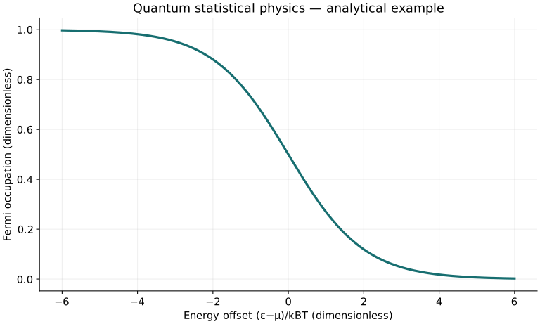
↑ Return to definitions and contentsGraphical worked example
Twenty worked examples
Open a problem to see its defined inputs, assumptions, equation, numerical substitution, result, and interpretation. Values are illustrative analytical exercises.
Example 01. Fermi occupation atμ
Definitions & inputs. x0.
Choose the governing model and isolate the requested quantity.
Insert the stated inputs in consistent units or the explicitly defined normalized units.
Evaluate the expression; the result uses the units shown.
Interpretation. Finite-temperature half occupation.
↑ Return to definitions and contentsExample 02. Fermi occupation aboveμ
Definitions & inputs. x1.
Choose the governing model and isolate the requested quantity.
Insert the stated inputs in consistent units or the explicitly defined normalized units.
Evaluate the expression; the result uses the units shown.
Interpretation. Dimensionless energy offset.
↑ Return to definitions and contentsExample 03. Fermi occupation belowμ
Definitions & inputs. x−1.
Choose the governing model and isolate the requested quantity.
Insert the stated inputs in consistent units or the explicitly defined normalized units.
Evaluate the expression; the result uses the units shown.
Interpretation. Complements occupation at x1.
↑ Return to definitions and contentsExample 04. Bose occupation
Definitions & inputs. x1.
Choose the governing model and isolate the requested quantity.
Insert the stated inputs in consistent units or the explicitly defined normalized units.
Evaluate the expression; the result uses the units shown.
Interpretation. Positive boson energy offset.
↑ Return to definitions and contentsExample 05. Classical occupation
Definitions & inputs. x5.
Choose the governing model and isolate the requested quantity.
Insert the stated inputs in consistent units or the explicitly defined normalized units.
Evaluate the expression; the result uses the units shown.
Interpretation. Low occupancy approximation.
↑ Return to definitions and contentsExample 06. Fermi variance
Definitions & inputs. f.5.
Choose the governing model and isolate the requested quantity.
Insert the stated inputs in consistent units or the explicitly defined normalized units.
Evaluate the expression; the result uses the units shown.
Interpretation. Single mode Bernoulli occupation.
↑ Return to definitions and contentsExample 07. Bose variance
Definitions & inputs. n1.
Choose the governing model and isolate the requested quantity.
Insert the stated inputs in consistent units or the explicitly defined normalized units.
Evaluate the expression; the result uses the units shown.
Interpretation. Enhanced single mode fluctuation.
↑ Return to definitions and contentsExample 08. Fermion mode partition
Definitions & inputs. x1.
Choose the governing model and isolate the requested quantity.
Insert the stated inputs in consistent units or the explicitly defined normalized units.
Evaluate the expression; the result uses the units shown.
Interpretation. Mode occupancy zero or one.
↑ Return to definitions and contentsExample 09. Boson mode partition
Definitions & inputs. x1.
Choose the governing model and isolate the requested quantity.
Insert the stated inputs in consistent units or the explicitly defined normalized units.
Evaluate the expression; the result uses the units shown.
Interpretation. Convergent geometric series.
↑ Return to definitions and contentsExample 10. Oscillator energy
Definitions & inputs. ℏω1energy unit,kBT1same unit.
Choose the governing model and isolate the requested quantity.
Insert the stated inputs in consistent units or the explicitly defined normalized units.
Evaluate the expression; the result uses the units shown.
Interpretation. Includes zero-point energy.
↑ Return to definitions and contentsExample 11. Oscillator heat capacity
Definitions & inputs. xℏω/kBT1.
Choose the governing model and isolate the requested quantity.
Insert the stated inputs in consistent units or the explicitly defined normalized units.
Evaluate the expression; the result uses the units shown.
Interpretation. Quantum heat capacity.
↑ Return to definitions and contentsExample 12. Fermi wavevector
Definitions & inputs. n10²⁸/m³,gspin2.
Choose the governing model and isolate the requested quantity.
Insert the stated inputs in consistent units or the explicitly defined normalized units.
Evaluate the expression; the result uses the units shown.
Interpretation. Homogeneous3Dgas.
↑ Return to definitions and contentsExample 13. Fermi energy
Definitions & inputs. n10²⁸/m³,me9.1093837×10⁻³¹kg,ℏ1.054571817×10⁻³⁴SI.
Choose the governing model and isolate the requested quantity.
Insert the stated inputs in consistent units or the explicitly defined normalized units.
Evaluate the expression; the result uses the units shown.
Interpretation. SI joules converted to eV.
↑ Return to definitions and contentsExample 14. Fermi temperature
Definitions & inputs. EF2eV,kB8.617333262×10⁻⁵eV/K.
Choose the governing model and isolate the requested quantity.
Insert the stated inputs in consistent units or the explicitly defined normalized units.
Evaluate the expression; the result uses the units shown.
Interpretation. Energy scale not actual temperature.
↑ Return to definitions and contentsExample 15. Mean zero-temperature energy
Definitions & inputs. EF2eV.
Choose the governing model and isolate the requested quantity.
Insert the stated inputs in consistent units or the explicitly defined normalized units.
Evaluate the expression; the result uses the units shown.
Interpretation. Ideal non relativistic gas.
↑ Return to definitions and contentsExample 16. Degeneracy pressure
Definitions & inputs. n10²⁸/m³,EF2eV.
Choose the governing model and isolate the requested quantity.
Insert the stated inputs in consistent units or the explicitly defined normalized units.
Evaluate the expression; the result uses the units shown.
Interpretation. Chosen EF illustrates formula independently of the previous density calculation.
↑ Return to definitions and contentsExample 17. Density scaling ofEF
Definitions & inputs. Doublen.
Choose the governing model and isolate the requested quantity.
Insert the stated inputs in consistent units or the explicitly defined normalized units.
Evaluate the expression; the result uses the units shown.
Interpretation. Fixed mass and degeneracy.
↑ Return to definitions and contentsExample 18. Condensate fraction
Definitions & inputs. T/Tc.5.
Choose the governing model and isolate the requested quantity.
Insert the stated inputs in consistent units or the explicitly defined normalized units.
Evaluate the expression; the result uses the units shown.
Interpretation. Uniform ideal3D Bose gas.
↑ Return to definitions and contentsExample 19. Condensate threshold phase-space density
Definitions & inputs. z1.
Choose the governing model and isolate the requested quantity.
Insert the stated inputs in consistent units or the explicitly defined normalized units.
Evaluate the expression; the result uses the units shown.
Interpretation. Thermodynamic ideal-gas limit.
↑ Return to definitions and contentsExample 20. Photon occupation
Definitions & inputs. hν/kBT2,μ0.
Choose the governing model and isolate the requested quantity.
Insert the stated inputs in consistent units or the explicitly defined normalized units.
Evaluate the expression; the result uses the units shown.
Interpretation. Per photon mode.
↑ Return to definitions and contentsSymbols and units
Each derivation and problem defines its own symbols and inputs. Symbols may be reused with different meanings in other subjects. Keep units consistent, retain sufficient precision during calculation, and apply the stated validity limits.