PHYSICS / ENGINEERING / COMPUTING
Survivability under environmental stresses and faults
Model civil engineering system survival against uncertain loads, thermal exposure, wear, interruption and shared faults, with twenty examples.
Matter pathway: atom → solid → liquid → gas → plasma. Quantum mechanics and quantum field theory provide foundations across the pathway; they are not additional phases. This is a connected modeling route, not a universal heating curve. Actual phases depend on pressure, composition, and kinetics.
1. Load-strength margin
Definitions & inputs. C capacity,L demand,g=C−L margin,μ and σ means and standard deviations.
Define success before assigning any probability.
Propagate the difference including dependence.
A Gaussian margin converts standardized separation into survival probability.
Interpretation. Tail extrapolation and an incorrect capacity model can dominate the result.
↑ Return to definitions and contents2. Hazards and common causes
Definitions & inputs. H discrete environmental scenario,Ps survival conditional on H,pcc shared disabling-event probability.
Average conditional survival over the actual exposure distribution.
A parallel pair is defeated by the shared event or both independent residual failures.
Multiply conditional probabilities, not unconditional ones when dependence exists.
Interpretation. Redundancy benefits depend on separation of shared power, environment, software and other common causes.
↑ Return to definitions and contents3. Accumulated exposure
Definitions & inputs. ni cycles at level i,Ni fitted cycles to failure,μ attenuation coefficient,x thickness,D dose.
Miner’s index accumulates fractions of fitted fatigue life.
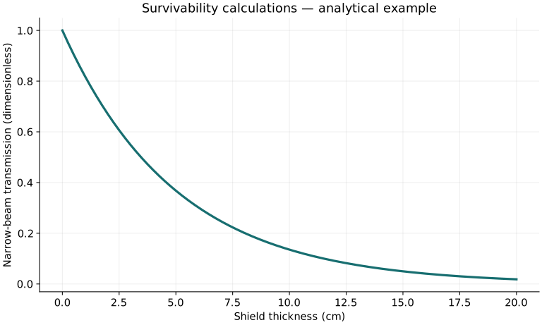
Independent removal per unit path gives exponential attenuation.
Solve the attenuation law for one-half transmission.
Interpretation. Miner’s D=1 is an approximate criterion; radiation buildup and spectral changes are excluded from the narrow-beam law.
↑ Return to definitions and contents4. Continuity and recovery
Definitions & inputs. E usable backup energy,P load,td detection,ts switching,tr recovery duration.
Stored usable energy supports a constant power load for a finite time.
Sequential detection and switching create a service interruption.
Integrate fractional lost function q(t) over recovery.
Interpretation. A system can survive physically while its service is unavailable; state both acceptance criteria.
↑ Return to definitions and contentsGraphical worked example
Twenty worked examples
Open a problem to see its defined inputs, assumptions, equation, numerical substitution, result, and interpretation. Values are illustrative analytical exercises.
Example 01. Capacity margin
Definitions & inputs. Capacity 150 N,demand 100 N.
Choose the governing model and isolate the requested quantity.
Insert the stated inputs in consistent units or the explicitly defined normalized units.
Evaluate the expression; the result uses the units shown.
Interpretation. Positive margin only addresses the defined load and failure mode.
↑ Return to definitions and contentsExample 02. Capacity-to-demand ratio
Definitions & inputs. Capacity 150 N,demand 100 N.
Choose the governing model and isolate the requested quantity.
Insert the stated inputs in consistent units or the explicitly defined normalized units.
Evaluate the expression; the result uses the units shown.
Interpretation. A ratio is not a survival probability.
↑ Return to definitions and contentsExample 03. Normalized reserve
Definitions & inputs. Capacity 150 N,demand 100 N.
Choose the governing model and isolate the requested quantity.
Insert the stated inputs in consistent units or the explicitly defined normalized units.
Evaluate the expression; the result uses the units shown.
Interpretation. This convention expresses reserve relative to demand.
↑ Return to definitions and contentsExample 04. Independent margin deviation
Definitions & inputs. σC=3 N,σL=4 N.
Choose the governing model and isolate the requested quantity.
Insert the stated inputs in consistent units or the explicitly defined normalized units.
Evaluate the expression; the result uses the units shown.
Interpretation. Correlated loads and capacity require a covariance term.
↑ Return to definitions and contentsExample 05. Standardized margin
Definitions & inputs. μC=120 N,μL=100 N,σg=10 N.
Choose the governing model and isolate the requested quantity.
Insert the stated inputs in consistent units or the explicitly defined normalized units.
Evaluate the expression; the result uses the units shown.
Interpretation. β is a reliability index under this normal-margin model.
↑ Return to definitions and contentsExample 06. Gaussian survival
Definitions & inputs. Margin mean 20 N,standard deviation 10 N.
Choose the governing model and isolate the requested quantity.
Insert the stated inputs in consistent units or the explicitly defined normalized units.
Evaluate the expression; the result uses the units shown.
Interpretation. The result depends on normal tails and the validity of the threshold model.
↑ Return to definitions and contentsExample 07. Scenario-weighted survival
Definitions & inputs. Mild scenario probability .8 with survival .99; severe probability .2 with survival .8.
Choose the governing model and isolate the requested quantity.
Insert the stated inputs in consistent units or the explicitly defined normalized units.
Evaluate the expression; the result uses the units shown.
Interpretation. The two scenarios are exhaustive and mutually exclusive.
↑ Return to definitions and contentsExample 08. Shared-fault parallel pair
Definitions & inputs. Shared disabling probability .02; conditional unit reliability .9 independent otherwise.
Choose the governing model and isolate the requested quantity.
Insert the stated inputs in consistent units or the explicitly defined normalized units.
Evaluate the expression; the result uses the units shown.
Interpretation. The shared event prevents the independent-pair result of .99.
↑ Return to definitions and contentsExample 09. Sequential-stage survival
Definitions & inputs. Stage1 survival .95; conditional stage2 survival given stage1 .9.
Choose the governing model and isolate the requested quantity.
Insert the stated inputs in consistent units or the explicitly defined normalized units.
Evaluate the expression; the result uses the units shown.
Interpretation. Conditional input handles dependence between stages.
↑ Return to definitions and contentsExample 10. Narrow-beam transmission
Definitions & inputs. μ=.2 cm⁻¹,thickness 5 cm.
Choose the governing model and isolate the requested quantity.
Insert the stated inputs in consistent units or the explicitly defined normalized units.
Evaluate the expression; the result uses the units shown.
Interpretation. Single energy, narrow beam and no buildup are assumed.
↑ Return to definitions and contentsExample 11. Half-value thickness
Definitions & inputs. μ=.2 cm⁻¹.
Choose the governing model and isolate the requested quantity.
Insert the stated inputs in consistent units or the explicitly defined normalized units.
Evaluate the expression; the result uses the units shown.
Interpretation. Material and photon energy determine the attenuation coefficient.
↑ Return to definitions and contentsExample 12. Exposure time to dose threshold
Definitions & inputs. Defined device limit 100 Gy,constant absorbed dose rate .5 Gy/h.
Choose the governing model and isolate the requested quantity.
Insert the stated inputs in consistent units or the explicitly defined normalized units.
Evaluate the expression; the result uses the units shown.
Interpretation. This hypothetical device threshold is not a human exposure guideline.
↑ Return to definitions and contentsExample 13. Cumulative fatigue index
Definitions & inputs. 1000 cycles at N1=10000;2000 at N2=20000.
Choose the governing model and isolate the requested quantity.
Insert the stated inputs in consistent units or the explicitly defined normalized units.
Evaluate the expression; the result uses the units shown.
Interpretation. Linear damage ignores sequence effects and scatter in fatigue life.
↑ Return to definitions and contentsExample 14. Remaining illustrative fatigue cycles
Definitions & inputs. Current D=.2;future cycles at fitted N=10000 until D=1.
Choose the governing model and isolate the requested quantity.
Insert the stated inputs in consistent units or the explicitly defined normalized units.
Evaluate the expression; the result uses the units shown.
Interpretation. This is a Miner-rule estimate, not a guaranteed remaining life.
↑ Return to definitions and contentsExample 15. Adiabatic thermal buffer
Definitions & inputs. Heat capacity 1000 J/K,allowed rise 20 K,net heat input 100 W.
Choose the governing model and isolate the requested quantity.
Insert the stated inputs in consistent units or the explicitly defined normalized units.
Evaluate the expression; the result uses the units shown.
Interpretation. No heat rejection occurs in this bound.
↑ Return to definitions and contentsExample 16. Cold-start temperature margin
Definitions & inputs. Predicted minimum −15°C,qualified minimum −20°C.
Choose the governing model and isolate the requested quantity.
Insert the stated inputs in consistent units or the explicitly defined normalized units.
Evaluate the expression; the result uses the units shown.
Interpretation. The relevant qualification applies to the actual startup condition.
↑ Return to definitions and contentsExample 17. Backup-energy hold time
Definitions & inputs. Usable energy 500 Wh,critical load 100 W.
Choose the governing model and isolate the requested quantity.
Insert the stated inputs in consistent units or the explicitly defined normalized units.
Evaluate the expression; the result uses the units shown.
Interpretation. Conversion losses are already included in usable energy.
↑ Return to definitions and contentsExample 18. Detection plus switchover gap
Definitions & inputs. Detection 20 ms,subsequent switch 5 ms.
Choose the governing model and isolate the requested quantity.
Insert the stated inputs in consistent units or the explicitly defined normalized units.
Evaluate the expression; the result uses the units shown.
Interpretation. The function must tolerate the full interruption.
↑ Return to definitions and contentsExample 19. Linear recovery lost-service time
Definitions & inputs. Function rises linearly from zero to full in 4 h.
Choose the governing model and isolate the requested quantity.
Insert the stated inputs in consistent units or the explicitly defined normalized units.
Evaluate the expression; the result uses the units shown.
Interpretation. This equals two hours of complete loss spread over a four-hour recovery.
↑ Return to definitions and contentsExample 20. Two independent exposure intervals
Definitions & inputs. Survival .98 in each interval with the stated independence.
Choose the governing model and isolate the requested quantity.
Insert the stated inputs in consistent units or the explicitly defined normalized units.
Evaluate the expression; the result uses the units shown.
Interpretation. Aging and accumulated damage often make independence inappropriate.
↑ Return to definitions and contentsSymbols and units
Each derivation and problem defines its own symbols and inputs. Symbols may be reused with different meanings in other subjects. Keep units consistent, retain sufficient precision during calculation, and apply the stated validity limits.