Ray tracing for optics and radiation heat transfer

1. Geometry: intersect, select the nearest surface, reflect or refract

Definitions & inputs. o is a ray origin, d a unit propagation vector, t a forward distance, n a unit surface normal, p a point on a plane. θ is measured from the interface normal; n1 and n2 are refractive indices.

1. Parameterize the ray in world coordinates.

   $$\mathbf x(t)=\mathbf o+t\mathbf d,\quad t>0$$

2. Insert the ray into the plane equation and solve. Among all valid surface hits use the nearest positive t.

   $$\mathbf n\cdot(\mathbf x-\mathbf p)=0\ \Rightarrow\ t=\frac{\mathbf n\cdot(\mathbf p-\mathbf o)}{\mathbf n\cdot\mathbf d}$$

3. Reverse the normal component and preserve the tangential component for specular reflection.

   $$\mathbf d_r=\mathbf d-2(\mathbf d\cdot\mathbf n)\mathbf n$$

4. Continuity of tangential wavevector gives Snell’s law; there is no propagating transmitted ray when the required sine exceeds one.

   $$n_1\sin\theta_i=n_2\sin\theta_t$$

5. At normal incidence between nonabsorbing dielectric media this Fresnel result gives reflected power fraction. Oblique rays need polarization-dependent Fresnel coefficients.

   $$R_0=\left(\frac{n_1-n_2}{n_1+n_2}\right)^2$$

Interpretation. Lens barrels, mirrors, imaging systems and solar concentrators need direction plus power accounting. Pure ray geometry does not reproduce interference or diffraction; use wave optics when those effects determine performance.

• pbrt — Specular reflection and transmission ↗

2. Radiometry and Monte Carlo path weights

Definitions & inputs. L radiance [W/(m² sr)], E irradiation [W/m²], J radiosity [W/m²], fr BRDF [sr⁻¹], ω direction, n normal. Φ is power [W]. A probability density pω is per steradian.

1. Projected area connects radiance to irradiance. Radiance is directional; it is not interchangeable with heat flux.

   $$d\Phi=L\cos\theta\,dA\,d\omega,\quad E=\int_{\Omega^+}L_i\cos\theta\,d\omega$$

2. Outgoing light is emitted plus reflected incident light, with the BRDF distributing directions.

   $$L_o(\omega_o)=L_e(\omega_o)+\int_{\Omega^+}f_r(\omega_i,\omega_o)L_i(\omega_i)\cos\theta_i\,d\omega_i$$

3. Importance sampling turns the integral into an estimator; omitting its probability-density denominator biases energy.

   $$\widehat L_o=L_e+\frac1N\sum_{m=1}^N\frac{f_r(\omega_m,\omega_o)L_i(\omega_m)\cos\theta_m}{p_\omega(\omega_m)}$$

4. For a Lambertian surface, cosine-weighted sampling leaves a simple reflectance factor per bounce.

   $$f_r=\rho/\pi,\quad p_\omega=\cos\theta/\pi\ \Rightarrow\ f_r\cos\theta/p_\omega=\rho$$

5. A homogeneous absorbing medium attenuates a ray by Beer–Lambert. Scattering also redirects energy and requires a volume-transport model.

   $$I(s)=I_0e^{-\kappa s}$$

Interpretation. Use optical solar absorptance for sunlight and thermal infrared emissivity for emitted heat; they are generally different band averages. Kirchhoff’s equality applies at matched wavelength, direction and thermodynamic conditions.

• pbrt — Light transport and surface reflection ↗

3. View factors: geometric probability before absorption

Definitions & inputs. Fij is the fraction of diffuse power leaving area Ai that first reaches Aj. Rij is point separation, θi and θj use inward-facing normals, V is binary visibility. ε is emissivity and does not enter a geometric view factor.

1. Convert a receiving area to solid angle and integrate cosine-weighted diffuse emission over the source.

   $$F_{ij}=\frac1{A_i}\int_{A_i}\int_{A_j}\frac{V\cos\theta_i\cos\theta_j}{\pi R_{ij}^2}\,dA_j\,dA_i$$

2. Swapping the two differential areas proves reciprocity. Closure holds for a complete enclosure, including any environment surface.

   $$A_iF_{ij}=A_jF_{ji},\quad\sum_jF_{ij}=1$$

3. Sample each source point uniformly by area and each launch direction with a cosine-weighted hemisphere density.

   $$\phi=2\pi u,\quad\cos\theta=\sqrt{1-v},\quad u,v\sim U[0,1]$$

4. Count first-hit rays. The standard-error expression is an independent-ray binomial approximation, not a systematic mesh-error estimate.

   $$\widehat F_{ij}=N_{i\to j}/N_i,\quad s_{\widehat F}\simeq\sqrt{\widehat F(1-\widehat F)/N_i}$$

Interpretation. Check nonnegativity, row sums, reciprocity and convergence. Independent noisy rows do not satisfy reciprocity exactly; any correction must preserve nonnegativity and closure jointly. A convex isolated surface has Fii=0, while a concave patch can see itself.

• NASA — Thermal Radiation Heat Transfer, enclosure analysis of Gebhart ↗

4. Gebhart absorption factors: sum every reflection path

Definitions & inputs. Bij is the fraction of radiation originally emitted by patch i that is ultimately absorbed by patch j, including reflections. Standard spelling is Gebhart (sometimes entered as “Gebhard”). E=diag(εj), R=diag(1−εj), F is the row-source view-factor matrix.

1. First paths hit j and are absorbed directly. All other contributions first hit k, reflect, and eventually end at j.

   $$B_{ij}=F_{ij}\epsilon_j+\sum_kF_{ik}(1-\epsilon_k)B_{kj}$$

2. The reflection probability belongs to the surface first hit, hence R multiplies F on its right. Matrix order matters.

   $$B=FE+FRB\ \Rightarrow\ (I-FR)B=FE$$

3. Expand into direct absorption, one prior reflection, two prior reflections, and so on when the series converges.

   $$B=FE+(FR)FE+(FR)^2FE+\cdots$$

4. Eventual absorption conserves energy; reciprocal diffuse-gray exchange has an emissivity-weighted reciprocity relation.

   $$\sum_jB_{ij}=1,\quad A_i\epsilon_iB_{ij}=A_j\epsilon_jB_{ji}$$

5. Worked closed two-surface example: B12=0.8/(1−0.2²)=5/6 and B11=0.2B21=1/6. Self-absorption can be nonzero even though F11=0.

   $$F=\begin{pmatrix}0&1\\1&0\end{pmatrix},\quad \epsilon_1=\epsilon_2=0.8\ \Rightarrow\ B=\begin{pmatrix}1/6&5/6\\5/6&1/6\end{pmatrix}$$

Interpretation. Solve the linear system rather than explicitly forming a matrix inverse. Direct path tracing can instead count final absorption events (or accumulated absorbed weights). Its Bij must converge to this solve for the same diffuse-gray geometry.

• NASA — Thermal Radiation Heat Transfer, enclosure analysis of Gebhart ↗

5. RadK: from absorption to a symmetric thermal network

Definitions & inputs. Qi is net power leaving node i. σ=5.670374419×10⁻⁸ W/(m² K⁴). Here Cij=Ai εi Bij has units m² and Kij=σCij has units W/K⁴. All temperatures in fourth powers are absolute kelvin.

1. Subtract incoming absorbed emissions from patch i’s own emitted power; its reflected self-return is included in the sum.

   $$Q_i=A_i\epsilon_i\sigma T_i^4-\sum_jA_j\epsilon_j\sigma B_{ji}T_j^4$$

2. Use absorption closure and weighted reciprocity to obtain pairwise exchange. The self term cancels.

   $$Q_i=\sum_jK_{ij}(T_i^4-T_j^4),\quad K_{ij}=\sigma A_i\epsilon_iB_{ij}=K_{ji}$$

3. Continue the two-surface example. The extra ε1 belongs to original emission; do not multiply again by ε2, already contained in B12.

   $$A_1=A_2=1\,\mathrm{m^2},\ \epsilon=0.8:\quad C_{12}=2/3\,\mathrm{m^2},\quad K_{12}=3.780249613\times10^{-8}\,\mathrm{W\,K^{-4}}$$

4. Evaluate the nonlinear exchange; the opposite node receives equal and opposite power.

   $$T_1=400\,\mathrm K,\ T_2=300\,\mathrm K:\quad Q_{12}=K_{12}(400^4-300^4)=661.5437\,\mathrm W$$

5. Factor the difference of fourth powers. This exact secant conductance is in W/K, not W/K⁴.

   $$G_{sec}=K_{ij}(T_i+T_j)(T_i^2+T_j^2),\quad Q_{ij}=G_{sec}(T_i-T_j)$$

6. A small-signal conductance is valid near a common reference temperature. The full Newton Jacobian uses ∂Qij/∂Ti=4KijTi³ and ∂Qij/∂Tj=−4KijTj³.

   $$T_i\simeq T_j\simeq T_0:\quad G_{lin}=4K_{ij}T_0^3$$

Interpretation. Never enter Celsius into T⁴ or multiply by the Stefan–Boltzmann constant twice. In a thermal energy balance, outward Qi is a loss: Ci dTi/dt=Pi−Qi plus conductive and other exchanges. External collimated solar heating is a source term, not automatically a symmetric thermal RadK.

• NASA — Thermal Radiation Heat Transfer, enclosure analysis of Gebhart ↗

6. Independent radiosity check and practical workflow

Definitions & inputs. Ji is outgoing radiosity and Hi incident irradiation, both W/m². b denotes a spectral band. Thermal Desktop/RadCAD is a practical example of software calculating form factors, radiation conductors and environmental heating.

1. Outgoing flux contains emitted and reflected incident flux.

   $$H_i=\sum_jF_{ij}J_j,\quad J_i=\epsilon_i\sigma T_i^4+(1-\epsilon_i)H_i$$

2. Assemble a second linear system. Note RF here versus FR in the Gebhart solve: the unknown radiosity and its source convention differ.

   $$(I-RF)\mathbf J=E\sigma\mathbf T^{\circ4}$$

3. This independent route must agree with the Gebhart heat balance for identical inputs.

   $$Q_i=A_i(J_i-H_i)$$

4. Check enclosure energy conservation and zero exchange at uniform temperature.

   $$\sum_iQ_i=0,\quad T_i=T_0\ \forall i\Rightarrow Q_i=0$$

5. For suitable reciprocal bandwise models, integrate blackbody emissive power over each band and use its consistent exchange coefficient; a single constant gray coefficient cannot represent arbitrary spectral properties.

   $$Q_{ij}=\sum_b C_{ij,b}\,[E_{b,b}(T_i)-E_{b,b}(T_j)]$$

Interpretation. Workflow: mesh and orient surfaces; assign measured band properties; trace and converge geometric or full absorption transport; enforce/check physical invariants; solve B or radiosity; export clearly labeled coefficient units; couple the energy balance; compare with black-body and two-plate benchmarks. RadCAD supports Monte Carlo ray tracing and radiosity; pbrt provides inspectable optical light-transport implementations.

• C&R Technologies — RadCAD radiation modeling capabilities ↗

Graphical worked example

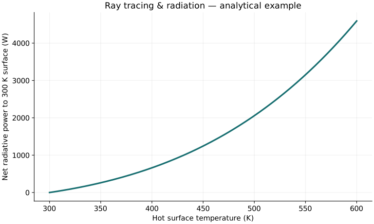
Twenty worked examples

Open a problem to see its defined inputs, assumptions, equation, numerical substitution, result, and interpretation. Values are illustrative analytical exercises.

Connect this subject to other models

• Optics models
• Heat transfer models
• Satellite design models
• Sensor types, measurement models and calibration

Return to the subject library · Numerical solution techniques

Typical sensors and experimental connections

Photodiode · Thermopile infrared sensor · Bolometer / microbolometer

These are examples of instruments used to measure relevant observables, calibrate parameters, or test a physical system. They do not directly measure every abstract model quantity or prove a theory by themselves. Choose bandwidth, range, environment and uncertainty for the actual experiment.

Explore the dedicated Sensors site →

Mathematical tools and foundations

Geometric series and convergence · Linear systems and elimination · Monte Carlo estimation

Use the stated mathematical conditions together with the physical assumptions. Explore the Mathematics atlas →