PHYSICS / ENGINEERING / COMPUTING
Hypersonic vehicle design: civil aerothermodynamics
Study high-speed atmospheric flight through regime selection, compressible flow, aerodynamic loads, thermal protection and verification.
Matter pathway: atom → solid → liquid → gas → plasma. Quantum mechanics and quantum field theory provide foundations across the pathway; they are not additional phases. This is a connected modeling route, not a universal heating curve. Actual phases depend on pressure, composition, and kinetics.
1. Choose the physical regime
Definitions & inputs. M Mach number,V velocity,a sound speed,Kn mean free path/body length,Re Reynolds number.
Compare flow speed with acoustic propagation.
Viscous and rarefaction scales determine whether continuum Navier–Stokes is appropriate.
Total enthalpy measures the available stagnation energy even when constant gamma fails.
Interpretation. High enthalpy may excite vibration, dissociate or ionize gas; use chemical nonequilibrium and rarefied-flow methods when the corresponding scales demand them.
↑ Return to definitions and contents2. Compression and stagnation limits
Definitions & inputs. T0 stagnation temperature,γ heat capacity ratio,M1 upstream normal Mach.
Combine h=cpT with total enthalpy conservation.
Normal-shock momentum and energy balance produce a pressure jump.
Mass conservation and the equation of state give compression; entropy rises across the shock.
Interpretation. Oblique and curved shocks need local geometry and a multidimensional solution; shock interactions and transition can create localized heating.
↑ Return to definitions and contents3. Loads and aerodynamic tradeoffs
Definitions & inputs. q dynamic pressure,S reference area,CL andCD coefficients,θ surface inclination.
Reference area and coefficient definitions must match.
Newtonian momentum transfer is a rough pressure model on windward surfaces, not a full viscous solution.
Lift-to-drag ratio connects aerodynamic forces but does not determine heating or vehicle feasibility.
Interpretation. Shape, structure, thermal protection, stability and propulsion interact; CFD requires mesh, chemistry, turbulence and wind-tunnel validation.
↑ Return to definitions and contents4. Thermal protection and model validation
Definitions & inputs. qdot incident heat flux,ε emissivity,σSB constant,Twall surface temperature,mc thermal capacity,k conductivity.
Balance incoming heat, reradiation and conducted energy.
A radiative-equilibrium benchmark omits heat storage and conduction.
Fourier conduction and diffusion time compare through-thickness response with exposure time.
Interpretation. Real TPS needs temperature-dependent properties, surface chemistry, recession and bond line limits. Compare analytical checks, mesh/time convergence, ground tests and uncertainty before interpreting vehicle predictions.
↑ Return to definitions and contentsGraphical worked example
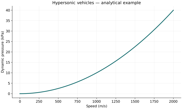
Twenty worked examples
Open a problem to see its defined inputs, assumptions, equation, numerical substitution, result, and interpretation. Values are illustrative analytical exercises.
Example 01. Sound speed
Definitions & inputs. γ1.4,R287J/(kgK),T220K.
Choose the governing model and isolate the requested quantity.
Insert the stated inputs in consistent units or the explicitly defined normalized units.
Evaluate the expression; the result uses the units shown.
Interpretation. Calorically perfect gas.
↑ Return to definitions and contentsExample 02. Mach number
Definitions & inputs. V1500m/s,a300m/s.
Choose the governing model and isolate the requested quantity.
Insert the stated inputs in consistent units or the explicitly defined normalized units.
Evaluate the expression; the result uses the units shown.
Interpretation. Regime indicator, not a heating prediction.
↑ Return to definitions and contentsExample 03. Specific kinetic energy
Definitions & inputs. V1500m/s.
Choose the governing model and isolate the requested quantity.
Insert the stated inputs in consistent units or the explicitly defined normalized units.
Evaluate the expression; the result uses the units shown.
Interpretation. Add static enthalpy for total enthalpy.
↑ Return to definitions and contentsExample 04. Perfect-gas stagnation ratio
Definitions & inputs. γ1.4,M5.
Choose the governing model and isolate the requested quantity.
Insert the stated inputs in consistent units or the explicitly defined normalized units.
Evaluate the expression; the result uses the units shown.
Interpretation. Chemistry and varying heat capacity omitted.
↑ Return to definitions and contentsExample 05. Perfect-gas stagnation temperature
Definitions & inputs. Static220K,ratio6.
Choose the governing model and isolate the requested quantity.
Insert the stated inputs in consistent units or the explicitly defined normalized units.
Evaluate the expression; the result uses the units shown.
Interpretation. Illustrative benchmark, not wall temperature.
↑ Return to definitions and contentsExample 06. Dynamic pressure
Definitions & inputs. ρ.02kg/m³,V1500m/s.
Choose the governing model and isolate the requested quantity.
Insert the stated inputs in consistent units or the explicitly defined normalized units.
Evaluate the expression; the result uses the units shown.
Interpretation. Local free-stream state.
↑ Return to definitions and contentsExample 07. Lift
Definitions & inputs. q22500Pa,S2m²,CL.2.
Choose the governing model and isolate the requested quantity.
Insert the stated inputs in consistent units or the explicitly defined normalized units.
Evaluate the expression; the result uses the units shown.
Interpretation. Assumed aerodynamic coefficient.
↑ Return to definitions and contentsExample 08. Drag
Definitions & inputs. q22500Pa,S2m²,CD.1.
Choose the governing model and isolate the requested quantity.
Insert the stated inputs in consistent units or the explicitly defined normalized units.
Evaluate the expression; the result uses the units shown.
Interpretation. Same reference area.
↑ Return to definitions and contentsExample 09. Lift-to-drag
Definitions & inputs. CL.2,CD.1.
Choose the governing model and isolate the requested quantity.
Insert the stated inputs in consistent units or the explicitly defined normalized units.
Evaluate the expression; the result uses the units shown.
Interpretation. At the specified operating point.
↑ Return to definitions and contentsExample 10. Drag power
Definitions & inputs. D4500N,V1500m/s.
Choose the governing model and isolate the requested quantity.
Insert the stated inputs in consistent units or the explicitly defined normalized units.
Evaluate the expression; the result uses the units shown.
Interpretation. Mechanical energy loss rate, not engine sizing.
↑ Return to definitions and contentsExample 11. Reynolds number
Definitions & inputs. ρ.02,V1500,L1m,μ1.5×10⁻⁵Pa·s.
Choose the governing model and isolate the requested quantity.
Insert the stated inputs in consistent units or the explicitly defined normalized units.
Evaluate the expression; the result uses the units shown.
Interpretation. Viscous regime indicator.
↑ Return to definitions and contentsExample 12. Knudsen number
Definitions & inputs. Mean free path10⁻⁵m,L.1m.
Choose the governing model and isolate the requested quantity.
Insert the stated inputs in consistent units or the explicitly defined normalized units.
Evaluate the expression; the result uses the units shown.
Interpretation. Continuum applicability also depends on local gradients.
↑ Return to definitions and contentsExample 13. Normal shock pressure ratio
Definitions & inputs. M5,γ1.4.
Choose the governing model and isolate the requested quantity.
Insert the stated inputs in consistent units or the explicitly defined normalized units.
Evaluate the expression; the result uses the units shown.
Interpretation. Ideal-gas normal shock.
↑ Return to definitions and contentsExample 14. Normal shock density ratio
Definitions & inputs. Same upstream.
Choose the governing model and isolate the requested quantity.
Insert the stated inputs in consistent units or the explicitly defined normalized units.
Evaluate the expression; the result uses the units shown.
Interpretation. Strong-shock perfect-gas limit is6 forγ1.4.
↑ Return to definitions and contentsExample 15. Normal shock temperature ratio
Definitions & inputs. Pressure29,density5.
Choose the governing model and isolate the requested quantity.
Insert the stated inputs in consistent units or the explicitly defined normalized units.
Evaluate the expression; the result uses the units shown.
Interpretation. Same gas constant on both sides.
↑ Return to definitions and contentsExample 16. Newtonian pressure coefficient
Definitions & inputs. Inclination30°.
Choose the governing model and isolate the requested quantity.
Insert the stated inputs in consistent units or the explicitly defined normalized units.
Evaluate the expression; the result uses the units shown.
Interpretation. Rough windward pressure approximation.
↑ Return to definitions and contentsExample 17. Stored-heat rise
Definitions & inputs. Heat100kJ,m10kg,cp1000J/(kgK).
Choose the governing model and isolate the requested quantity.
Insert the stated inputs in consistent units or the explicitly defined normalized units.
Evaluate the expression; the result uses the units shown.
Interpretation. No concurrent cooling.
↑ Return to definitions and contentsExample 18. Radiative equilibrium
Definitions & inputs. Heat flux100000W/m²,ε.8,σ5.670374419×10⁻⁸.
Choose the governing model and isolate the requested quantity.
Insert the stated inputs in consistent units or the explicitly defined normalized units.
Evaluate the expression; the result uses the units shown.
Interpretation. No conduction or heat storage in this estimate.
↑ Return to definitions and contentsExample 19. Conduction heat flux
Definitions & inputs. k.1W/(mK),ΔT500K,L.05m.
Choose the governing model and isolate the requested quantity.
Insert the stated inputs in consistent units or the explicitly defined normalized units.
Evaluate the expression; the result uses the units shown.
Interpretation. Constant-property planar conduction.
↑ Return to definitions and contentsExample 20. Diffusion timescale
Definitions & inputs. L.05m,α10⁻⁷m²/s.
Choose the governing model and isolate the requested quantity.
Insert the stated inputs in consistent units or the explicitly defined normalized units.
Evaluate the expression; the result uses the units shown.
Interpretation. Order-of-magnitude diffusion time, not exact TPS transient.
↑ Return to definitions and contentsSymbols and units
Each derivation and problem defines its own symbols and inputs. Symbols may be reused with different meanings in other subjects. Keep units consistent, retain sufficient precision during calculation, and apply the stated validity limits.