PHYSICS / ENGINEERING / COMPUTING
Heat transfer models
Build from energy conservation to conduction, convection, radiation, transient cooling and heat exchangers, with twenty worked examples.
Matter pathway: atom → solid → liquid → gas → plasma. Quantum mechanics and quantum field theory provide foundations across the pathway; they are not additional phases. This is a connected modeling route, not a universal heating curve. Actual phases depend on pressure, composition, and kinetics.
1. Conduction and energy balance
Definitions & inputs. k conductivity,ρ density,cp heat capacity,T temperature,qdot volumetric generation.
Fourier’s law sends heat down the temperature gradient.
Balance energy storage against conduction and generation.
Integrate the steady one-dimensional no-generation equation across a slab.
Interpretation. Composite walls add series resistances when the same heat rate crosses each layer.
↑ Return to definitions and contents2. Surface exchange
Definitions & inputs. h convection coefficient,A area,ε emissivity,σ Stefan–Boltzmann constant.
Define convection through the surface-to-fluid temperature difference.
Subtract absorbed enclosure irradiation from emitted radiation.
Factor the fourth-power difference to obtain a temperature-dependent linearized coefficient.
Interpretation. View factors and interacting finite surfaces require a radiation network.
↑ Return to definitions and contents3. Transient cooling
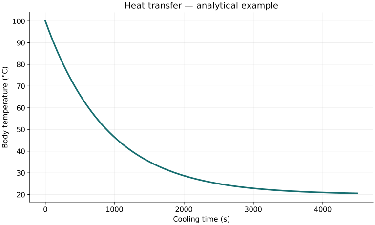
Definitions & inputs. Lc=V/A,α=k/(ρcp),Bi Biot number,θ=T−T∞.
Compare internal conduction resistance with surface resistance and define thermal time.
Apply an energy balance to the uniform body.
Integrate from the initial uniform temperature.
Interpretation. If Bi is large, solve spatial conduction with appropriate geometry and boundary conditions.
↑ Return to definitions and contents4. Fins and exchangers
Definitions & inputs. m fin parameter,k conductivity,P perimeter,Ac cross section; Cdot heat-capacity rate.
Solve the fin conduction-convection equation with the insulated-tip boundary condition.
Integrate the stream energy balance.
Integration along an ideal parallel or counterflow exchanger gives the log-mean driving difference.
Interpretation. Multipass geometry and phase changes need the corresponding exchanger formulation.
↑ Return to definitions and contentsGraphical worked example
Twenty worked examples
Open a problem to see its defined inputs, assumptions, equation, numerical substitution, result, and interpretation. Values are illustrative analytical exercises.
Example 01. Plane-wall heat flow
Definitions & inputs. k=.5 W/(m K),A=2 m²,L=.1 m,ΔT=20 K.
Choose the governing model and isolate the requested quantity.
Insert the stated inputs in consistent units or the explicitly defined normalized units.
Evaluate the expression; the result uses the units shown.
Interpretation. Steady one-dimensional conduction excludes edge losses.
↑ Return to definitions and contentsExample 02. Wall thermal resistance
Definitions & inputs. k=.5 W/(m K),A=2 m²,L=.1 m.
Choose the governing model and isolate the requested quantity.
Insert the stated inputs in consistent units or the explicitly defined normalized units.
Evaluate the expression; the result uses the units shown.
Interpretation. Multiply resistance by heat rate to obtain temperature drop.
↑ Return to definitions and contentsExample 03. Series wall flow
Definitions & inputs. R1=.1,R2=.2 K/W,total ΔT=30 K.
Choose the governing model and isolate the requested quantity.
Insert the stated inputs in consistent units or the explicitly defined normalized units.
Evaluate the expression; the result uses the units shown.
Interpretation. The same heat rate passes through both layers.
↑ Return to definitions and contentsExample 04. Convection heat flow
Definitions & inputs. h=10 W/(m² K),A=2 m²,Ts−T∞=30 K.
Choose the governing model and isolate the requested quantity.
Insert the stated inputs in consistent units or the explicitly defined normalized units.
Evaluate the expression; the result uses the units shown.
Interpretation. The convection coefficient is a prescribed input.
↑ Return to definitions and contentsExample 05. Convection resistance
Definitions & inputs. h=20 W/(m² K),A=.5 m².
Choose the governing model and isolate the requested quantity.
Insert the stated inputs in consistent units or the explicitly defined normalized units.
Evaluate the expression; the result uses the units shown.
Interpretation. Fouling and contact resistances are additional elements.
↑ Return to definitions and contentsExample 06. Net thermal radiation
Definitions & inputs. ε=.8,A=1 m²,Ts=400 K,Tsur=300 K,σ=5.670374419×10⁻⁸.
Choose the governing model and isolate the requested quantity.
Insert the stated inputs in consistent units or the explicitly defined normalized units.
Evaluate the expression; the result uses the units shown.
Interpretation. Large enclosure, view factor one, and gray diffuse behavior are assumed.
↑ Return to definitions and contentsExample 07. Linearized radiation coefficient
Definitions & inputs. Same ε=.8,Ts=400 K,Tsur=300 K.
Choose the governing model and isolate the requested quantity.
Insert the stated inputs in consistent units or the explicitly defined normalized units.
Evaluate the expression; the result uses the units shown.
Interpretation. Multiplying by 100 K reproduces the net radiation heat flux.
↑ Return to definitions and contentsExample 08. Sensible heating energy
Definitions & inputs. m=2 kg,cp=900 J/(kg K),ΔT=50 K.
Choose the governing model and isolate the requested quantity.
Insert the stated inputs in consistent units or the explicitly defined normalized units.
Evaluate the expression; the result uses the units shown.
Interpretation. No phase change or environmental loss is included.
↑ Return to definitions and contentsExample 09. Heating time
Definitions & inputs. Required energy 90 kJ,net constant heater power 300 W.
Choose the governing model and isolate the requested quantity.
Insert the stated inputs in consistent units or the explicitly defined normalized units.
Evaluate the expression; the result uses the units shown.
Interpretation. Net power already subtracts heat losses.
↑ Return to definitions and contentsExample 10. Thermal diffusivity
Definitions & inputs. k=200 W/(m K),ρ=2700 kg/m³,cp=900 J/(kg K).
Choose the governing model and isolate the requested quantity.
Insert the stated inputs in consistent units or the explicitly defined normalized units.
Evaluate the expression; the result uses the units shown.
Interpretation. Diffusivity sets the rate of temperature spreading.
↑ Return to definitions and contentsExample 11. Biot number
Definitions & inputs. h=10 W/(m² K),Lc=.01 m,k=200 W/(m K).
Choose the governing model and isolate the requested quantity.
Insert the stated inputs in consistent units or the explicitly defined normalized units.
Evaluate the expression; the result uses the units shown.
Interpretation. The small value supports a lumped-temperature approximation.
↑ Return to definitions and contentsExample 12. Lumped thermal time
Definitions & inputs. m=1 kg,cp=900 J/(kg K),h=10 W/(m² K),A=.1 m².
Choose the governing model and isolate the requested quantity.
Insert the stated inputs in consistent units or the explicitly defined normalized units.
Evaluate the expression; the result uses the units shown.
Interpretation. Verify a small Biot number separately.
↑ Return to definitions and contentsExample 13. Temperature after one time constant
Definitions & inputs. T0=100°C,T∞=20°C,t=τ.
Choose the governing model and isolate the requested quantity.
Insert the stated inputs in consistent units or the explicitly defined normalized units.
Evaluate the expression; the result uses the units shown.
Interpretation. Temperature differences may be in Celsius for this nonradiative relation.
↑ Return to definitions and contentsExample 14. Cooling to ten-percent excess
Definitions & inputs. τ=900 s,θ/θ0=.1.
Choose the governing model and isolate the requested quantity.
Insert the stated inputs in consistent units or the explicitly defined normalized units.
Evaluate the expression; the result uses the units shown.
Interpretation. Ambient temperature is held constant.
↑ Return to definitions and contentsExample 15. Fourier number
Definitions & inputs. α=10⁻⁵ m²/s,t=100 s,L=.1 m.
Choose the governing model and isolate the requested quantity.
Insert the stated inputs in consistent units or the explicitly defined normalized units.
Evaluate the expression; the result uses the units shown.
Interpretation. Length convention must match the geometry-specific transient solution.
↑ Return to definitions and contentsExample 16. Cylindrical conduction
Definitions & inputs. k=1 W/(m K),L=1 m,r1=.01 m,r2=.02 m,ΔT=20 K.
Choose the governing model and isolate the requested quantity.
Insert the stated inputs in consistent units or the explicitly defined normalized units.
Evaluate the expression; the result uses the units shown.
Interpretation. Steady radial flow has area increasing with radius.
↑ Return to definitions and contentsExample 17. Fin efficiency
Definitions & inputs. Straight insulated-tip fin with mL=1.
Choose the governing model and isolate the requested quantity.
Insert the stated inputs in consistent units or the explicitly defined normalized units.
Evaluate the expression; the result uses the units shown.
Interpretation. Fin efficiency compares actual heat loss with a fin uniformly at base temperature.
↑ Return to definitions and contentsExample 18. Stream heating
Definitions & inputs. Mass flow .1 kg/s,cp=4200 J/(kg K),rise 10 K.
Choose the governing model and isolate the requested quantity.
Insert the stated inputs in consistent units or the explicitly defined normalized units.
Evaluate the expression; the result uses the units shown.
Interpretation. The heat-capacity approximation is constant over the temperature range.
↑ Return to definitions and contentsExample 19. Log-mean temperature difference
Definitions & inputs. End driving differences 40 K and 20 K.
Choose the governing model and isolate the requested quantity.
Insert the stated inputs in consistent units or the explicitly defined normalized units.
Evaluate the expression; the result uses the units shown.
Interpretation. Both differences use consistent hot-minus-cold terminal temperatures.
↑ Return to definitions and contentsExample 20. Latent melting energy
Definitions & inputs. m=.5 kg,latent heat 334 kJ/kg; already at melting point.
Choose the governing model and isolate the requested quantity.
Insert the stated inputs in consistent units or the explicitly defined normalized units.
Evaluate the expression; the result uses the units shown.
Interpretation. Sensible preheating and postheating are separate terms.
↑ Return to definitions and contentsSymbols and units
Each derivation and problem defines its own symbols and inputs. Symbols may be reused with different meanings in other subjects. Keep units consistent, retain sufficient precision during calculation, and apply the stated validity limits.