Quantum computing models

1. Qubits, gates, and measurement

Definitions & inputs. |ψ⟩=α|0⟩+β|1⟩; α,β complex amplitudes. Basis ordering for two qubits is |q0 q1⟩.

1. The Born rule maps amplitudes to measurement probabilities.

   $$|\alpha|^2+|\beta|^2=1,\quad P(1)=|\beta|^2$$

2. Unitary gates preserve normalization.

   $$|\psi^\prime\rangle=U|\psi\rangle,\quad U^\dagger U=I$$

3. Matrix multiplication gives a tunable measurement probability.

   $$R_y(\theta)|0\rangle=\cos(\theta/2)|0\rangle+\sin(\theta/2)|1\rangle$$

Interpretation. Global phase is unobservable; relative phase can affect later measurements.

• IBM Quantum Learning — quantum information and circuits ↗

2. Bell states and density matrices

Definitions & inputs. ρ is a density operator; Tr traces over a basis; ZA,ZB are Pauli-Z observables on the two qubits.

1. A Hadamard and controlled-NOT prepare a Bell state.

   $$|00\rangle\xrightarrow{H\otimes I}(|00\rangle+|10\rangle)/\sqrt2\xrightarrow{\rm CNOT}(|00\rangle+|11\rangle)/\sqrt2$$

2. Each subsystem is maximally mixed although the joint state is pure.

   $$\rho_A=\operatorname{Tr}_B|\Phi^+\rangle\langle\Phi^+|=I/2$$

3. Local randomness coexists with perfect joint correlation.

   $$\langle Z_AZ_B\rangle=1,\quad\operatorname{Tr}\rho_A^2=1/2$$

Interpretation. Entanglement correlations do not permit faster-than-light signaling.

• IBM Quantum Learning — quantum information and circuits ↗

3. Interference in small algorithms

Definitions & inputs. N search items, one marked item; θ=arcsin(1/√N); r Grover iterations; m phase-estimation bits.

1. Two reflections rotate amplitude in the marked/unmarked subspace.

   $$P_{\rm Grover}(r)=\sin^2[(2r+1)\theta]$$

2. Controlled powers and inverse Fourier transform recover an exactly representable eigenphase on an exact eigenstate.

   $$U|u\rangle=e^{2\pi i\phi}|u\rangle,\quad k=2^m\phi\quad\text{when integer}$$

3. The Fourier transform changes phases; a basis input yields uniform computational-basis outcome probabilities.

   $$\mathrm{QFT}_N|j\rangle=N^{-1/2}\sum_{k=0}^{N-1}e^{2\pi ijk/N}|k\rangle$$

Interpretation. Algorithmic advantage depends on data access, oracle cost, errors, and classical alternatives.

• IBM Quantum Learning — quantum information and circuits ↗

4. Noise and finite-shot inference

Definitions & inputs. T1 is energy relaxation time, T2 phase-coherence time, nshots independent measurements, and p a measured-event probability.

1. Separate population loss from off-diagonal coherence.

   $$P_1(t)=P_1(0)e^{-t/T_1},\quad|\rho_{01}(t)|=|\rho_{01}(0)|e^{-t/T_2}$$

2. Pure dephasing adds to the coherence decay rate in this simple model.

   $$1/T_2=1/(2T_1)+1/T_\phi$$

3. A binomial model gives sampling uncertainty, distinct from device bias.

   $$\sigma_{\hat p}=\sqrt{p(1-p)/n_{\rm shots}}$$

Interpretation. A simulator result is not a hardware validation; real error budgets include preparation, gates, readout, and correlations.

• IBM Quantum Learning — quantum information and circuits ↗

5. Algorithm foundations: reversible queries and phase kickback

Definitions & inputs. x is an n-bit candidate, f(x) is a Boolean predicate, ⊕ is addition modulo two, |−⟩=(|0⟩−|1⟩)/√2. An oracle is a reversible circuit computing the predicate, not a source that reveals the answer for free.

1. Store the predicate in a target qubit while preserving the candidate, which makes the map reversible.

   $$U_f|x\rangle|b\rangle=|x\rangle|b\oplus f(x)\rangle$$

2. The minus state is an eigenstate of the bit-flip gate with eigenvalue −1.

   $$X|{-}\rangle=-|{-}\rangle$$

3. A controlled bit flip therefore becomes a phase on the candidate. The ancilla separates from the data.

   $$U_f|x\rangle|{-}\rangle=(-1)^{f(x)}|x\rangle|{-}\rangle$$

4. Hadamard gates prepare equal amplitudes. An immediate measurement still returns a uniformly random candidate.

   $$|s\rangle=H^{\otimes n}|0^n\rangle=\frac1{\sqrt N}\sum_{x=0}^{N-1}|x\rangle,\quad N=2^n$$

Interpretation. Algorithms create useful interference before measurement. They do not provide simultaneous classical access to all amplitudes. Oracle synthesis and data loading contribute real cost.

• Grover — A fast quantum mechanical algorithm for database search ↗

6. Grover: derive the two-reflection rotation

Definitions & inputs. N candidates contain M marked answers, 0<M<N. |G⟩ and |B⟩ are normalized uniform superpositions of good and bad candidates. θ=arcsin√(M/N). Basis ordering below is (|G⟩, |B⟩).

1. Group equal candidate amplitudes into a two-dimensional subspace.

   $$|s\rangle=\sqrt{M/N}|G\rangle+\sqrt{1-M/N}|B\rangle=\sin\theta|G\rangle+\cos\theta|B\rangle$$

2. Within this subspace the oracle reflects the good component. On the full space its projector includes every marked basis state.

   $$O=I-2|G\rangle\langle G|=\begin{pmatrix}-1&0\\0&1\end{pmatrix}$$

3. Expand the outer product. The diffuser reflects about the initial state.

   $$D=2|s\rangle\langle s|-I=\begin{pmatrix}-\cos2\theta&\sin2\theta\\\sin2\theta&\cos2\theta\end{pmatrix}$$

4. Apply the oracle first, then the diffuser: two reflections give a rotation toward the good axis.

   $$G=DO=\begin{pmatrix}\cos2\theta&\sin2\theta\\-\sin2\theta&\cos2\theta\end{pmatrix}$$

5. Multiply once and use the angle-addition identities; induction proves the expression for k iterations.

   $$G^k|s\rangle=\sin[(2k+1)\theta]|G\rangle+\cos[(2k+1)\theta]|B\rangle$$

6. Square the good amplitude. Compare neighboring nonnegative integers around k* to choose the first peak.

   $$P_k=\sin^2[(2k+1)\theta],\quad k_*\approx\frac{\pi}{4\theta}-\frac12$$

7. For sparse solutions this is a quadratic query improvement over classical unstructured search.

   $$\theta\simeq\sqrt{M/N}\ \Rightarrow\ k=O(\sqrt{N/M})$$

Interpretation. More iterations can reduce success: the state rotates past the good direction. Verify a measured candidate classically. Unknown M calls for an adaptive search or counting method; the quadratic oracle count does not remove the cost of implementing each oracle.

• Grover — A fast quantum mechanical algorithm for database search ↗

7. Grover worked examples: four and eight candidates

Definitions & inputs. First mark |11⟩ among four two-qubit strings. Amplitude vectors use order 00,01,10,11. Second use one marked answer among eight candidates.

1. For the two-qubit example a controlled-Z gate marks |11⟩.

   $$|s\rangle=\tfrac12(1,1,1,1)^{\mathsf T}\ \xrightarrow{O}\ \tfrac12(1,1,1,-1)^{\mathsf T}$$

2. The diffuser maps each amplitude to its reflection about the mean amplitude, not the mean probability.

   $$\bar a=\tfrac14(\tfrac12+\tfrac12+\tfrac12-\tfrac12)=\tfrac14,\quad a_x\xrightarrow{D}2\bar a-a_x$$

3. All unmarked amplitudes cancel and the target amplitude becomes one.

   $$DO|s\rangle=(0,0,0,1)^{\mathsf T},\quad P_1=1$$

4. The same derivation works beyond the special exact two-qubit case.

   $$N=8,\ M=1:\quad \theta=\arcsin(1/\sqrt8),\quad P_0=1/8$$

5. Two oracle queries give 94.53125% success in the eight-candidate example.

   $$P_1=\sin^2(3\theta)=25/32,\quad P_2=\sin^2(5\theta)=121/128$$

6. A third iteration overshoots and drops success to about 33.0%.

   $$P_3=\sin^2(7\theta)=169/512$$

Interpretation. The diffuser circuit is H⊗n(2|0…0⟩⟨0…0|−I)H⊗n. A circuit implementing the negative of this operator differs only by a global phase for ordinary Grover search. Relative and global phase must not be confused.

• Grover — A fast quantum mechanical algorithm for database search ↗

8. Quantum Fourier transform and phase estimation

Definitions & inputs. U|u⟩=exp(2πiφ)|u⟩ with 0≤φ<1. A t-qubit control register has Q=2ᵗ states. y is the measured integer. This derivation uses the inverse QFT sign convention shown.

1. Initialize a uniform control superposition and the target eigenstate.

   $$|0^t\rangle|u\rangle\xrightarrow{H^{\otimes t}}\frac1{\sqrt Q}\sum_{x=0}^{Q-1}|x\rangle|u\rangle$$

2. Controlled U, U², U⁴, … combine according to the binary digits of x. Eigenphase is kicked back to the control register.

   $$\frac1{\sqrt Q}\sum_x|x\rangle U^x|u\rangle=\frac1{\sqrt Q}\sum_x e^{2\pi i x\phi}|x\rangle|u\rangle$$

3. The inverse transform converts a phase gradient into an integer peak.

   $$F_Q^{-1}|x\rangle=\frac1{\sqrt Q}\sum_{y=0}^{Q-1}e^{-2\pi ixy/Q}|y\rangle$$

4. Collect the amplitude of output y.

   $$A(y)=\frac1Q\sum_{x=0}^{Q-1}e^{2\pi ix(\phi-y/Q)}$$

5. Sum the geometric series and take its squared magnitude, using the limiting value at removable singularities.

   $$P(y)=\frac{\sin^2[\pi Q(\phi-y/Q)]}{Q^2\sin^2[\pi(\phi-y/Q)]}$$

6. A worked exact phase produces the bit string 011 under the stated integer ordering; other grid outputs vanish.

   $$\phi=3/8,\ Q=8\ \Rightarrow\ P(y=3)=1$$

Interpretation. When Qφ is not an integer, nearby outcomes have nonzero probability. A standard exact t-qubit QFT uses Hadamards, controlled phase rotations of angles π/2, π/4, …, and final swaps; its inverse reverses gate order and phase signs. The gate count is O(t²), excluding controlled-U synthesis.

• Shor — Polynomial-Time Algorithms for Prime Factorization and Discrete Logarithms ↗

9. Shor: reduce factoring to order finding

Definitions & inputs. N is an odd composite integer after classical checks for even numbers and perfect powers. Choose 1<a<N coprime to N. The order r is the least positive integer satisfying aʳ≡1 mod N.

1. Run Euclid’s classical algorithm first; only a coprime base needs quantum order finding.

   $$d=\gcd(a,N)>1\ \Rightarrow\ d\text{ is already a nontrivial factor}$$

2. Factor a difference of squares after obtaining an even order.

   $$a^r\equiv1\pmod N,\quad r\text{ even}\ \Rightarrow\ (a^{r/2}-1)(a^{r/2}+1)\equiv0\pmod N$$

3. A nontrivial square root of one can separate factors of N.

   $$x=a^{r/2}\bmod N,\quad x\not\equiv\pm1\pmod N$$

4. The gcd extracts divisors without requiring a quantum measurement to return the factors directly.

   $$d_- =\gcd(x-1,N),\quad d_+=\gcd(x+1,N)$$

5. Verify each proposed divisor. Repeat the base selection if the order is odd or the square root is trivial.

   $$1<d_{\pm}<N,\quad N\bmod d_{\pm}=0$$

Interpretation. Shor’s speedup concerns a structured arithmetic problem. The quantum component estimates a period; modular arithmetic and continued fractions do the classical postprocessing. Factoring arbitrary large cryptographic integers also requires sufficiently accurate, fault-tolerant hardware.

• Shor — Polynomial-Time Algorithms for Prime Factorization and Discrete Logarithms ↗

10. Shor: derive the order-finding eigenstates and period readout

Definitions & inputs. Ua maps |y⟩ to |ay mod N⟩ for 0≤y<N and acts as identity on unused computational basis states. Since gcd(a,N)=1 this is a permutation. |us⟩ labels eigenphases s/r for s=0,…,r−1.

1. Superpose the cyclic orbit of one with Fourier phases.

   $$|u_s\rangle=\frac1{\sqrt r}\sum_{k=0}^{r-1}e^{-2\pi isk/r}|a^k\bmod N\rangle$$

2. Shift k to k+1, relabel the cyclic sum, and factor out exp(2πis/r).

   $$U_a|u_s\rangle=e^{2\pi is/r}|u_s\rangle$$

3. Fourier orthogonality cancels every orbit basis state except k=0. A simple target initialization therefore supplies a uniform eigenphase mixture for measurement.

   $$|1\rangle=\frac1{\sqrt r}\sum_{s=0}^{r-1}|u_s\rangle$$

4. Controlled modular powers a^(2ʲ) implement the phase-estimation interaction without enumerating every x classically.

   $$\frac1{\sqrt Q}\sum_x|x\rangle|1\rangle\ \xrightarrow{\mathrm{modular\ exponentiation}}\ \frac1{\sqrt Q}\sum_x|x\rangle|a^x\bmod N\rangle$$

5. Use the preceding phase-estimation derivation. An ideal experiment samples different s values; it does not always return 1/r.

   $$F_Q^{-1}\text{ on controls}\quad\Rightarrow\quad y/Q\approx s/r$$

6. A sufficiently close sample permits rational reconstruction. The nearest-grid outcome with Q≥N² satisfies this error bound, but not every measurement is nearest-grid.

   $$\left|\frac yQ-\frac sr\right|<\frac1{2r^2}\quad\Rightarrow\quad\text{the reduced }s/r\text{ is a continued-fraction convergent}$$

7. Test candidate denominators, appropriate multiples, or combine samples and rerun. A shared factor gcd(s,r)>1 can produce only a divisor of the true order.

   $$\hat r\text{ candidate}:\quad a^{\hat r}\bmod N\stackrel{?}=1$$

Interpretation. The order must be validated before taking gcds. A sample y=0 is uninformative. Efficient reversible modular exponentiation and the QFT give polynomial scaling in log N; this is not a claim that a tiny demonstration circuit scales directly to useful factoring.

• Shor — Polynomial-Time Algorithms for Prime Factorization and Discrete Logarithms ↗

11. Shor worked example: factor 15, including failed samples

Definitions & inputs. N=15, a=2, Q=256 (eight control qubits); four target qubits encode residues. In the ideal arithmetic circuit the order is r=4.

1. List this small orbit to check the result independently: the first return occurs after four steps.

   $$2^0,2^1,2^2,2^3,2^4\pmod{15}=1,2,4,8,1$$

2. All four phases lie exactly on the Q=256 grid, so each listed output has probability 1/4.

   $$\phi\in\{0,1/4,1/2,3/4\}\ \Rightarrow\ y\in\{0,64,128,192\}$$

3. The continued fraction immediately supplies denominator four, which passes the order test.

   $$y=64:\quad 64/256=1/4=[0;4]\ \Rightarrow\ \hat r=4,\quad 2^4\bmod15=1$$

4. The two gcds recover 15=3×5.

   $$x=2^{4/2}=4,\quad\gcd(4-1,15)=3,\quad\gcd(4+1,15)=5$$

5. The reduced fraction loses a factor of two in the denominator. Test a multiple or gather another sample; do not call two the order.

   $$y=128:\quad 128/256=1/2,\quad 2^2\bmod15=4\ne1$$

6. Even a correct order can fail the factor-extraction condition for a poor base. For a=14 both gcd outputs are trivial.

   $$y=0\text{ is uninformative};\quad a=14:\ r=2,\ a^{r/2}\equiv-1\pmod{15}$$

Interpretation. For this example, the two coprime phase numerators 1 and 3 directly yield the full order, together with probability 1/2. Verification and repeated sampling are part of the algorithm, not optional repairs.

• Shor — Polynomial-Time Algorithms for Prime Factorization and Discrete Logarithms ↗

Graphical worked example

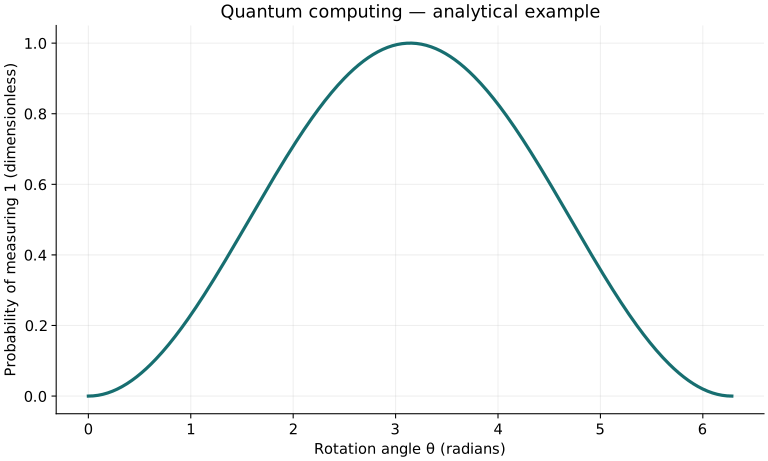
Twenty worked examples

Open a problem to see its defined inputs, assumptions, equation, numerical substitution, result, and interpretation. Values are illustrative analytical exercises.

Connect this subject to other models

• Quantum mechanics: atoms to matter
• Quantum field theory: fields to matter
• Microelectronics models
• Computer chip design models

Return to the subject library · Numerical solution techniques

Typical sensors and experimental connections

Single-photon avalanche diode (SPAD) · Photomultiplier tube · SQUID magnetometer

These are examples of instruments used to measure relevant observables, calibrate parameters, or test a physical system. They do not directly measure every abstract model quantity or prove a theory by themselves. Choose bandwidth, range, environment and uncertainty for the actual experiment.

Explore the dedicated Sensors site →

Mathematical tools and foundations

Modular arithmetic and orders

Use the stated mathematical conditions together with the physical assumptions. Explore the Mathematics atlas →