PHYSICS / ENGINEERING / COMPUTING
Operating systems and computer science models
Understand CPU scheduling, virtual memory, concurrency costs, storage, and queues through derivations and twenty worked examples.
Matter pathway: atom → solid → liquid → gas → plasma. Quantum mechanics and quantum field theory provide foundations across the pathway; they are not additional phases. This is a connected modeling route, not a universal heating curve. Actual phases depend on pressure, composition, and kinetics.
1. CPU scheduling metrics
Definitions & inputs. A arrival time, F completion time, C service time, S first start; all on one time axis.
Measure completion delay and first-service delay separately.
Remove actual CPU service to obtain ready-queue wait in this model.
Average over the stated job population, not over arbitrary clock samples.
Interpretation. First-come scheduling and shortest-job scheduling trade fairness and mean delay.
↑ Return to definitions and contents2. Virtual memory and caches
Definitions & inputs. P page size, a virtual address, h TLB hit probability, tT TLB access, tM memory access.
Split an address into page index and within-page offset.
Weight the hit and miss paths.
Rare disk-backed faults may dominate the average latency.
Interpretation. Multilevel walks, caches, and overlap change the latency model.
↑ Return to definitions and contents3. Concurrency and scaling
Definitions & inputs. s serial fraction, N parallel workers, E efficiency, a per-operation overhead.
Only the parallel portion benefits from more workers.
Invert normalized time and compare to linear speedup.
Context-switch overhead accumulates with switch frequency.
Interpretation. Contention, synchronization, coherence, and imbalance can reduce speedup further.
↑ Return to definitions and contents4. Storage and queues
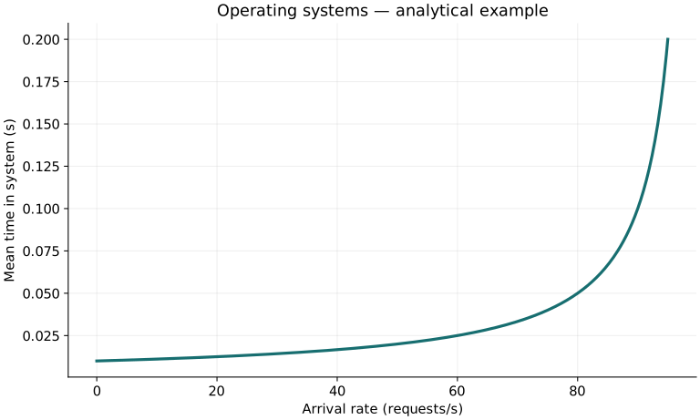
Definitions & inputs. λ arrivals/s, μ service completions/s, W mean system time, L mean jobs in system.
Queueing delay grows as utilization approaches unity.
Little’s law applies more broadly to stable systems with consistent boundaries.
A simple rotating-disk model adds positioning and sequential transfer.
Interpretation. Solid-state storage has different latency mechanisms; do not reuse disk rotation formulas there.
↑ Return to definitions and contentsGraphical worked example
Twenty worked examples
Open a problem to see its defined inputs, assumptions, equation, numerical substitution, result, and interpretation. Values are illustrative analytical exercises.
Example 01. Turnaround time
Definitions & inputs. Job arrives at 3 ms and finishes at 15 ms.
Choose the governing model and isolate the requested quantity.
Insert the stated inputs in consistent units or the explicitly defined normalized units.
Evaluate the expression; the result uses the units shown.
Interpretation. This includes queueing and service.
↑ Return to definitions and contentsExample 02. Response time
Definitions & inputs. Job arrives at 3 ms; first scheduled at 7 ms.
Choose the governing model and isolate the requested quantity.
Insert the stated inputs in consistent units or the explicitly defined normalized units.
Evaluate the expression; the result uses the units shown.
Interpretation. Response time is not completion time.
↑ Return to definitions and contentsExample 03. Waiting time
Definitions & inputs. Turnaround 12 ms, CPU burst 5 ms, no blocked time.
Choose the governing model and isolate the requested quantity.
Insert the stated inputs in consistent units or the explicitly defined normalized units.
Evaluate the expression; the result uses the units shown.
Interpretation. Subtract blocked intervals too if they are present.
↑ Return to definitions and contentsExample 04. FCFS mean waiting
Definitions & inputs. Three jobs arrive at zero with bursts 6,2,1 ms, in that order.
Choose the governing model and isolate the requested quantity.
Insert the stated inputs in consistent units or the explicitly defined normalized units.
Evaluate the expression; the result uses the units shown.
Interpretation. Nonpreemptive FCFS retains arrival order.
↑ Return to definitions and contentsExample 05. Shortest-job mean waiting
Definitions & inputs. Same simultaneous bursts sorted 1,2,6 ms.
Choose the governing model and isolate the requested quantity.
Insert the stated inputs in consistent units or the explicitly defined normalized units.
Evaluate the expression; the result uses the units shown.
Interpretation. Burst lengths are assumed known in advance.
↑ Return to definitions and contentsExample 06. Round-robin overhead
Definitions & inputs. Useful quantum 4 ms; switch cost 0.1 ms each quantum.
Choose the governing model and isolate the requested quantity.
Insert the stated inputs in consistent units or the explicitly defined normalized units.
Evaluate the expression; the result uses the units shown.
Interpretation. This assumes a switch after every quantum.
↑ Return to definitions and contentsExample 07. Context-switch CPU share
Definitions & inputs. 5000 switches/s, 2 μs cost each.
Choose the governing model and isolate the requested quantity.
Insert the stated inputs in consistent units or the explicitly defined normalized units.
Evaluate the expression; the result uses the units shown.
Interpretation. Cache refill costs are not included unless measured in the switch cost.
↑ Return to definitions and contentsExample 08. Virtual page number
Definitions & inputs. Byte address 12345, page size 4096 bytes.
Choose the governing model and isolate the requested quantity.
Insert the stated inputs in consistent units or the explicitly defined normalized units.
Evaluate the expression; the result uses the units shown.
Interpretation. Page numbering starts at zero.
↑ Return to definitions and contentsExample 09. Page offset
Definitions & inputs. Byte address 12345, page size 4096 bytes.
Choose the governing model and isolate the requested quantity.
Insert the stated inputs in consistent units or the explicitly defined normalized units.
Evaluate the expression; the result uses the units shown.
Interpretation. The offset is unchanged by ordinary page translation.
↑ Return to definitions and contentsExample 10. Page-table storage
Definitions & inputs. 32-bit byte virtual space, 4 KiB pages, 4-byte entry, flat table.
Choose the governing model and isolate the requested quantity.
Insert the stated inputs in consistent units or the explicitly defined normalized units.
Evaluate the expression; the result uses the units shown.
Interpretation. Sparse multilevel tables can consume much less for sparse mappings.
↑ Return to definitions and contentsExample 11. Mean final-page waste
Definitions & inputs. Uniform positive allocation remainder across a 4096-byte page; continuous approximation.
Choose the governing model and isolate the requested quantity.
Insert the stated inputs in consistent units or the explicitly defined normalized units.
Evaluate the expression; the result uses the units shown.
Interpretation. Exact discrete-byte averaging differs by half a byte.
↑ Return to definitions and contentsExample 12. TLB effective access
Definitions & inputs. Hit probability .99, TLB 1 ns, memory 100 ns; serial lookup and one-level walk.
Choose the governing model and isolate the requested quantity.
Insert the stated inputs in consistent units or the explicitly defined normalized units.
Evaluate the expression; the result uses the units shown.
Interpretation. The model excludes overlapping lookup and page faults.
↑ Return to definitions and contentsExample 13. Page-fault effective latency
Definitions & inputs. Normal 100 ns; fault path total 10 ms; fault probability 10⁻⁶.
Choose the governing model and isolate the requested quantity.
Insert the stated inputs in consistent units or the explicitly defined normalized units.
Evaluate the expression; the result uses the units shown.
Interpretation. A very small fault probability still adds noticeable average cost.
↑ Return to definitions and contentsExample 14. Working-set footprint
Definitions & inputs. 200 resident pages, each 4 KiB.
Choose the governing model and isolate the requested quantity.
Insert the stated inputs in consistent units or the explicitly defined normalized units.
Evaluate the expression; the result uses the units shown.
Interpretation. Sharing can reduce distinct physical frames across processes.
↑ Return to definitions and contentsExample 15. Amdahl speedup
Definitions & inputs. Serial fraction .1, four workers.
Choose the governing model and isolate the requested quantity.
Insert the stated inputs in consistent units or the explicitly defined normalized units.
Evaluate the expression; the result uses the units shown.
Interpretation. This upper estimate omits parallel overhead.
↑ Return to definitions and contentsExample 16. Parallel efficiency
Definitions & inputs. Speedup 3 with 4 workers.
Choose the governing model and isolate the requested quantity.
Insert the stated inputs in consistent units or the explicitly defined normalized units.
Evaluate the expression; the result uses the units shown.
Interpretation. Efficiency is a ratio to ideal linear scaling.
↑ Return to definitions and contentsExample 17. Queue mean system time
Definitions & inputs. M/M/1 λ=80/s and μ=100/s.
Choose the governing model and isolate the requested quantity.
Insert the stated inputs in consistent units or the explicitly defined normalized units.
Evaluate the expression; the result uses the units shown.
Interpretation. The mean includes service, not only queue wait.
↑ Return to definitions and contentsExample 18. Mean outstanding requests
Definitions & inputs. Throughput 200/s, mean system time .03 s, stable queue.
Choose the governing model and isolate the requested quantity.
Insert the stated inputs in consistent units or the explicitly defined normalized units.
Evaluate the expression; the result uses the units shown.
Interpretation. The measurement boundary for L and W must match.
↑ Return to definitions and contentsExample 19. Disk mean rotational delay
Definitions & inputs. 7200 revolutions/minute; random arrival angle.
Choose the governing model and isolate the requested quantity.
Insert the stated inputs in consistent units or the explicitly defined normalized units.
Evaluate the expression; the result uses the units shown.
Interpretation. This applies to a rotating disk and excludes seek time.
↑ Return to definitions and contentsExample 20. Sequential transfer time
Definitions & inputs. 100 MB at 200 MB/s, decimal units; positioning excluded.
Choose the governing model and isolate the requested quantity.
Insert the stated inputs in consistent units or the explicitly defined normalized units.
Evaluate the expression; the result uses the units shown.
Interpretation. Controller, filesystem, and contention overhead may add latency.
↑ Return to definitions and contentsSymbols and units
Each derivation and problem defines its own symbols and inputs. Symbols may be reused with different meanings in other subjects. Keep units consistent, retain sufficient precision during calculation, and apply the stated validity limits.