PHYSICS / ENGINEERING / COMPUTING
Optics models
Derive ray, wave, diffraction, polarization, and detection models, then solve twenty optical design and measurement examples.
Matter pathway: atom → solid → liquid → gas → plasma. Quantum mechanics and quantum field theory provide foundations across the pathway; they are not additional phases. This is a connected modeling route, not a universal heating curve. Actual phases depend on pressure, composition, and kinetics.
1. Refraction and paraxial imaging
Definitions & inputs. n is refractive index, θ ray angle to the surface normal, s object distance, s′ image distance, f focal length.
Stationary optical path, or tangential wave-vector continuity, gives Snell’s law.
Linearize angles for paraxial rays.
Similar triangles and the thin-lens ray rules give the imaging equation and signed magnification.
Interpretation. A thin-lens approximation does not include aberrations or thickness.
↑ Return to definitions and contents2. Interference and coherence
Definitions & inputs. E1,E2 are complex field amplitudes; φ relative phase; I1,I2 intensities.
Intensity comes from the squared total field.
Optical-path difference Δ sets phase.
For two narrow slits separated by d in the far field, adjacent fringes differ by one wavelength of path.
Interpretation. Finite bandwidth and imperfect coherence reduce fringe visibility.
↑ Return to definitions and contents3. Apertures and Gaussian beams
Definitions & inputs. a is slit width, D circular pupil diameter, w0 Gaussian waist radius at 1/e² intensity, and zR Rayleigh range.
Integrate contributions across a uniform slit.
The slit zeros and circular-aperture first minimum set characteristic diffraction angles.
A Gaussian beam spreads with propagation; waist size and divergence are linked.
Interpretation. Diffraction sets a reference resolution, while sampling and aberrations can worsen it.
↑ Return to definitions and contents4. Polarization, attenuation, and photodetection
Definitions & inputs. θ is polarizer angle, α absorption coefficient, P optical power, η quantum efficiency, q elementary charge.
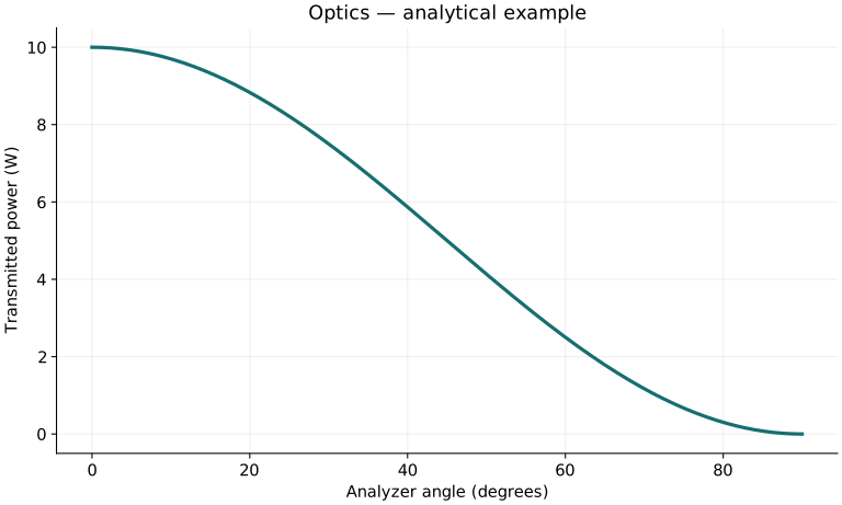
Project the electric field onto the analyzer axis, then square.
Integrate attenuation through a homogeneous path.
Photon energy converts power into photon rate and collected charge rate.
Interpretation. Detector dark current, read noise, and saturation require additional models.
↑ Return to definitions and contentsGraphical worked example
Twenty worked examples
Open a problem to see its defined inputs, assumptions, equation, numerical substitution, result, and interpretation. Values are illustrative analytical exercises.
Example 01. Refraction into glass
Definitions & inputs. n1=1, n2=1.5, θ1=30°.
Choose the governing model and isolate the requested quantity.
Insert the stated inputs in consistent units or the explicitly defined normalized units.
Evaluate the expression; the result uses the units shown.
Interpretation. The ray bends toward the normal.
↑ Return to definitions and contentsExample 02. Critical angle
Definitions & inputs. Light exits n1=1.5 glass into n2=1 air.
Choose the governing model and isolate the requested quantity.
Insert the stated inputs in consistent units or the explicitly defined normalized units.
Evaluate the expression; the result uses the units shown.
Interpretation. Larger incident angles permit total internal reflection.
↑ Return to definitions and contentsExample 03. Normal-incidence Fresnel reflection
Definitions & inputs. n1=1, n2=1.5.
Choose the governing model and isolate the requested quantity.
Insert the stated inputs in consistent units or the explicitly defined normalized units.
Evaluate the expression; the result uses the units shown.
Interpretation. Four percent of incident intensity reflects at one interface.
↑ Return to definitions and contentsExample 04. Image distance
Definitions & inputs. f=100 mm; s=300 mm.
Choose the governing model and isolate the requested quantity.
Insert the stated inputs in consistent units or the explicitly defined normalized units.
Evaluate the expression; the result uses the units shown.
Interpretation. The positive image distance is a real image.
↑ Return to definitions and contentsExample 05. Signed magnification
Definitions & inputs. s=300 mm; s′=150 mm.
Choose the governing model and isolate the requested quantity.
Insert the stated inputs in consistent units or the explicitly defined normalized units.
Evaluate the expression; the result uses the units shown.
Interpretation. The image is inverted and half-size.
↑ Return to definitions and contentsExample 06. Lens optical power
Definitions & inputs. f=0.25 m.
Choose the governing model and isolate the requested quantity.
Insert the stated inputs in consistent units or the explicitly defined normalized units.
Evaluate the expression; the result uses the units shown.
Interpretation. This is +4 dioptres.
↑ Return to definitions and contentsExample 07. Two-slit fringe spacing
Definitions & inputs. λ=500 nm, L=2 m, d=0.5 mm.
Choose the governing model and isolate the requested quantity.
Insert the stated inputs in consistent units or the explicitly defined normalized units.
Evaluate the expression; the result uses the units shown.
Interpretation. Adjacent bright fringes are 2 mm apart.
↑ Return to definitions and contentsExample 08. Interference at phase π/2
Definitions & inputs. I1=I2=1 W/m²; φ=π/2.
Choose the governing model and isolate the requested quantity.
Insert the stated inputs in consistent units or the explicitly defined normalized units.
Evaluate the expression; the result uses the units shown.
Interpretation. At quadrature the interference term vanishes.
↑ Return to definitions and contentsExample 09. Single-slit first minimum
Definitions & inputs. a=100 µm, λ=500 nm.
Choose the governing model and isolate the requested quantity.
Insert the stated inputs in consistent units or the explicitly defined normalized units.
Evaluate the expression; the result uses the units shown.
Interpretation. The central lobe extends between the positive and negative first minima.
↑ Return to definitions and contentsExample 10. Circular-aperture angular scale
Definitions & inputs. D=0.10 m, λ=550 nm.
Choose the governing model and isolate the requested quantity.
Insert the stated inputs in consistent units or the explicitly defined normalized units.
Evaluate the expression; the result uses the units shown.
Interpretation. This first-zero angle is about 1.38 arcseconds.
↑ Return to definitions and contentsExample 11. Airy radius at a focal plane
Definitions & inputs. f=0.20 m, D=0.05 m, λ=500 nm.
Choose the governing model and isolate the requested quantity.
Insert the stated inputs in consistent units or the explicitly defined normalized units.
Evaluate the expression; the result uses the units shown.
Interpretation. The first dark ring lies 2.44 µm from the centre.
↑ Return to definitions and contentsExample 12. Gaussian Rayleigh range
Definitions & inputs. w0=0.5 mm, λ=1 µm.
Choose the governing model and isolate the requested quantity.
Insert the stated inputs in consistent units or the explicitly defined normalized units.
Evaluate the expression; the result uses the units shown.
Interpretation. The beam area doubles at one Rayleigh range.
↑ Return to definitions and contentsExample 13. Gaussian beam radius
Definitions & inputs. w0=0.5 mm, z=2zR.
Choose the governing model and isolate the requested quantity.
Insert the stated inputs in consistent units or the explicitly defined normalized units.
Evaluate the expression; the result uses the units shown.
Interpretation. The reported radius uses 1/e² intensity.
↑ Return to definitions and contentsExample 14. Polarizer transmission
Definitions & inputs. I0=10 W/m², analyzer angle 60°.
Choose the governing model and isolate the requested quantity.
Insert the stated inputs in consistent units or the explicitly defined normalized units.
Evaluate the expression; the result uses the units shown.
Interpretation. The incident light is already linearly polarized.
↑ Return to definitions and contentsExample 15. Quarter-wave optical path
Definitions & inputs. λ=600 nm.
Choose the governing model and isolate the requested quantity.
Insert the stated inputs in consistent units or the explicitly defined normalized units.
Evaluate the expression; the result uses the units shown.
Interpretation. This optical-path difference produces π/2 phase delay.
↑ Return to definitions and contentsExample 16. Beer-law transmission
Definitions & inputs. α=2 m⁻¹, path l=0.3 m.
Choose the governing model and isolate the requested quantity.
Insert the stated inputs in consistent units or the explicitly defined normalized units.
Evaluate the expression; the result uses the units shown.
Interpretation. About 54.9% of intensity remains.
↑ Return to definitions and contentsExample 17. Photon energy at 500 nm
Definitions & inputs. hc=1239.841984 eV nm.
Choose the governing model and isolate the requested quantity.
Insert the stated inputs in consistent units or the explicitly defined normalized units.
Evaluate the expression; the result uses the units shown.
Interpretation. Optical power consists of many such photons per second.
↑ Return to definitions and contentsExample 18. Photon rate
Definitions & inputs. P=1 mW, λ=500 nm, h=6.62607015×10⁻³⁴ J s.
Choose the governing model and isolate the requested quantity.
Insert the stated inputs in consistent units or the explicitly defined normalized units.
Evaluate the expression; the result uses the units shown.
Interpretation. This is incident photon rate, not detected electron rate.
↑ Return to definitions and contentsExample 19. Photodiode current
Definitions & inputs. Incident photon rate 10¹² s⁻¹, η=0.8, q=1.602176634×10⁻¹⁹ C.
Choose the governing model and isolate the requested quantity.
Insert the stated inputs in consistent units or the explicitly defined normalized units.
Evaluate the expression; the result uses the units shown.
Interpretation. Quantum efficiency accounts for uncollected photons.
↑ Return to definitions and contentsExample 20. Shot-noise signal-to-noise
Definitions & inputs. N=10000 detected photoelectrons, negligible background.
Choose the governing model and isolate the requested quantity.
Insert the stated inputs in consistent units or the explicitly defined normalized units.
Evaluate the expression; the result uses the units shown.
Interpretation. Read noise and background would reduce SNR.
↑ Return to definitions and contentsSymbols and units
Each derivation and problem defines its own symbols and inputs. Symbols may be reused with different meanings in other subjects. Keep units consistent, retain sufficient precision during calculation, and apply the stated validity limits.