PHYSICS / ENGINEERING / COMPUTING
Statistics: probability, estimation and inference
Connect probability models to sampling, parameter estimation, intervals, regression and reproducible interpretation.
Matter pathway: atom → solid → liquid → gas → plasma. Quantum mechanics and quantum field theory provide foundations across the pathway; they are not additional phases. This is a connected modeling route, not a universal heating curve. Actual phases depend on pressure, composition, and kinetics.
1. Probability and moments
Definitions & inputs. X random variable,p probability mass,density f,μ mean,σ² variance.
Weighted outcomes define expectation and spread.
Transform the random variable and center its fluctuations.
Cross terms matter unless covariance is zero.
Interpretation. Zero correlation is weaker than independence; probabilities and densities have different units.
↑ Return to definitions and contents2. Sampling and estimation
Definitions & inputs. xi independent observations,n count,xbar sample mean,s² sample variance.
Fitting the sample mean consumes one degree of freedom, giving the unbiased variance denominator.
Independent sample variances add and the mean divides their sum byn².
Under normal sampling the statistic follows a t distribution withn−1 degrees of freedom under the stated null.
Interpretation. More observations reduce random sampling error but do not automatically remove selection bias or measurement offset.
↑ Return to definitions and contents3. Intervals and hypothesis tests
Definitions & inputs. α error rate,z or t quantile,μ unknown population mean.
A repeated-sampling normal interval has nominal coverage under its model.
Estimating variance broadens the critical value, especially for smalln.
A p-value is conditional on the null model; it is not the probability that the null is true.
Interpretation. Report effect sizes, uncertainty, selection of analyses and multiple-testing control, not only a significance label.
↑ Return to definitions and contents4. Regression and Bayesian updating
Definitions & inputs. y observations,X design matrix,β coefficients,ε errors,θ parameter,D data.
Differentiate squared residual loss and solve the normal equations; QR or SVD is preferable numerically.
Homoscedastic independent errors produce the familiar covariance; use other estimators when assumptions fail.
Bayes’ theorem updates a prior using the likelihood.
Interpretation. Confidence, prediction and credible intervals answer different questions; correlation or a fitted slope alone does not establish causation.
↑ Return to definitions and contentsGraphical worked example
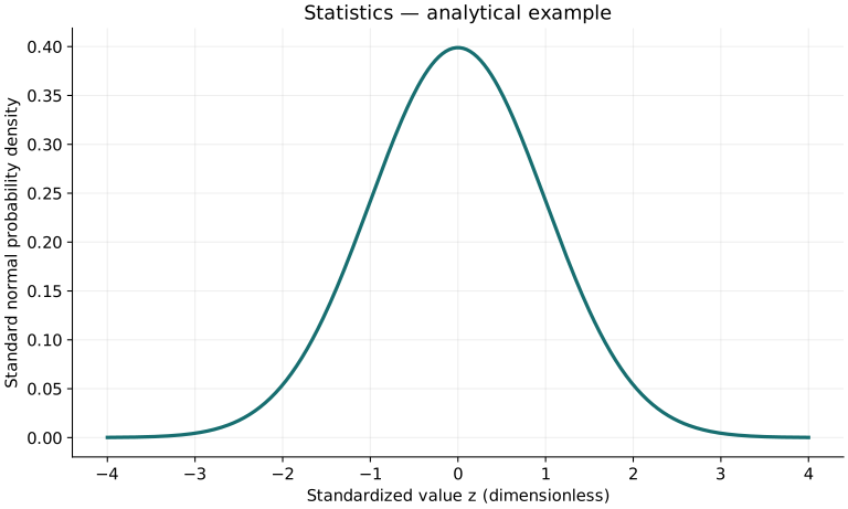
Twenty worked examples
Open a problem to see its defined inputs, assumptions, equation, numerical substitution, result, and interpretation. Values are illustrative analytical exercises.
Example 01. Mean
Definitions & inputs. Data2,4,6.
Choose the governing model and isolate the requested quantity.
Insert the stated inputs in consistent units or the explicitly defined normalized units.
Evaluate the expression; the result uses the units shown.
Interpretation. Arithmetic mean.
↑ Return to definitions and contentsExample 02. Sample variance
Definitions & inputs. Same data.
Choose the governing model and isolate the requested quantity.
Insert the stated inputs in consistent units or the explicitly defined normalized units.
Evaluate the expression; the result uses the units shown.
Interpretation. Usesn−1.
↑ Return to definitions and contentsExample 03. Sample standard deviation
Definitions & inputs. Variance4.
Choose the governing model and isolate the requested quantity.
Insert the stated inputs in consistent units or the explicitly defined normalized units.
Evaluate the expression; the result uses the units shown.
Interpretation. Same units as data.
↑ Return to definitions and contentsExample 04. Standard error
Definitions & inputs. σ2,n100.
Choose the governing model and isolate the requested quantity.
Insert the stated inputs in consistent units or the explicitly defined normalized units.
Evaluate the expression; the result uses the units shown.
Interpretation. Independent samples.
↑ Return to definitions and contentsExample 05. Known variance95percent half width
Definitions & inputs. SE.2,z1.959964.
Choose the governing model and isolate the requested quantity.
Insert the stated inputs in consistent units or the explicitly defined normalized units.
Evaluate the expression; the result uses the units shown.
Interpretation. Normal interval.
↑ Return to definitions and contentsExample 06. Normal z score
Definitions & inputs. x14,μ10,σ2.
Choose the governing model and isolate the requested quantity.
Insert the stated inputs in consistent units or the explicitly defined normalized units.
Evaluate the expression; the result uses the units shown.
Interpretation. Standardization.
↑ Return to definitions and contentsExample 07. Bernoulli variance
Definitions & inputs. p.3.
Choose the governing model and isolate the requested quantity.
Insert the stated inputs in consistent units or the explicitly defined normalized units.
Evaluate the expression; the result uses the units shown.
Interpretation. Binary outcome.
↑ Return to definitions and contentsExample 08. Binomial mean
Definitions & inputs. n20,p.3.
Choose the governing model and isolate the requested quantity.
Insert the stated inputs in consistent units or the explicitly defined normalized units.
Evaluate the expression; the result uses the units shown.
Interpretation. Independent identical trials.
↑ Return to definitions and contentsExample 09. Binomial variance
Definitions & inputs. Same.
Choose the governing model and isolate the requested quantity.
Insert the stated inputs in consistent units or the explicitly defined normalized units.
Evaluate the expression; the result uses the units shown.
Interpretation. Count variance.
↑ Return to definitions and contentsExample 10. Zero successes
Definitions & inputs. n5,p.2.
Choose the governing model and isolate the requested quantity.
Insert the stated inputs in consistent units or the explicitly defined normalized units.
Evaluate the expression; the result uses the units shown.
Interpretation. Binomial model.
↑ Return to definitions and contentsExample 11. Poisson zero count
Definitions & inputs. λ3.
Choose the governing model and isolate the requested quantity.
Insert the stated inputs in consistent units or the explicitly defined normalized units.
Evaluate the expression; the result uses the units shown.
Interpretation. E qui dispersed Poisson count.
↑ Return to definitions and contentsExample 12. Exponential mean
Definitions & inputs. Rate.2/s.
Choose the governing model and isolate the requested quantity.
Insert the stated inputs in consistent units or the explicitly defined normalized units.
Evaluate the expression; the result uses the units shown.
Interpretation. Memory less waiting time.
↑ Return to definitions and contentsExample 13. Uniform variance
Definitions & inputs. Uniform0to2.
Choose the governing model and isolate the requested quantity.
Insert the stated inputs in consistent units or the explicitly defined normalized units.
Evaluate the expression; the result uses the units shown.
Interpretation. Continuous distribution.
↑ Return to definitions and contentsExample 14. Independent sum variance
Definitions & inputs. Variances4and9.
Choose the governing model and isolate the requested quantity.
Insert the stated inputs in consistent units or the explicitly defined normalized units.
Evaluate the expression; the result uses the units shown.
Interpretation. Zero covariance.
↑ Return to definitions and contentsExample 15. Correlated sum variance
Definitions & inputs. σ12,σ23,correlation.5.
Choose the governing model and isolate the requested quantity.
Insert the stated inputs in consistent units or the explicitly defined normalized units.
Evaluate the expression; the result uses the units shown.
Interpretation. Co variance must be in units of product.
↑ Return to definitions and contentsExample 16. Slope
Definitions & inputs. Exact points(0,1),(1,3),(2,5).
Choose the governing model and isolate the requested quantity.
Insert the stated inputs in consistent units or the explicitly defined normalized units.
Evaluate the expression; the result uses the units shown.
Interpretation. Perfect linear illustration.
↑ Return to definitions and contentsExample 17. Intercept
Definitions & inputs. y1atx0,slope2.
Choose the governing model and isolate the requested quantity.
Insert the stated inputs in consistent units or the explicitly defined normalized units.
Evaluate the expression; the result uses the units shown.
Interpretation. Modely=a+bx.
↑ Return to definitions and contentsExample 18. Residual
Definitions & inputs. Observation5,prediction4.5.
Choose the governing model and isolate the requested quantity.
Insert the stated inputs in consistent units or the explicitly defined normalized units.
Evaluate the expression; the result uses the units shown.
Interpretation. Signed residual.
↑ Return to definitions and contentsExample 19. Beta-Binomial posterior mean
Definitions & inputs. Prior Beta1,1;7successes3failures.
Choose the governing model and isolate the requested quantity.
Insert the stated inputs in consistent units or the explicitly defined normalized units.
Evaluate the expression; the result uses the units shown.
Interpretation. Bayesian mean with uniform prior.
↑ Return to definitions and contentsExample 20. Bonferroni threshold
Definitions & inputs. Familyα.05,10tests.
Choose the governing model and isolate the requested quantity.
Insert the stated inputs in consistent units or the explicitly defined normalized units.
Evaluate the expression; the result uses the units shown.
Interpretation. Union-bound family wise control,not power optimal.
↑ Return to definitions and contentsSymbols and units
Each derivation and problem defines its own symbols and inputs. Symbols may be reused with different meanings in other subjects. Keep units consistent, retain sufficient precision during calculation, and apply the stated validity limits.