PHYSICS / ENGINEERING / COMPUTING
Car design: road loads, handling, ride and energy
Relate vehicle mass, tires, aerodynamics, gearing and suspension to longitudinal performance and basic handling.
Matter pathway: atom → solid → liquid → gas → plasma. Quantum mechanics and quantum field theory provide foundations across the pathway; they are not additional phases. This is a connected modeling route, not a universal heating curve. Actual phases depend on pressure, composition, and kinetics.
1. Longitudinal force balance
Definitions & inputs. m mass,a acceleration,V speed,ρ air density,CdA drag area,Crr rolling coefficient,θ road angle.
Aerodynamic drag and rolling loss oppose motion.
Newton’s law combines acceleration and road loads.
Convert wheel force to mechanical power at the road.
Interpretation. Rotational inertia, speed-dependent tire losses and accessories add terms to an energy-consumption model.
↑ Return to definitions and contents2. Gearing and traction
Definitions & inputs. Tm motor/engine torque,i ratio,η drive line efficiency,rw wheel radius,μ tire friction.
Mechanical gearing trades shaft speed for wheel torque.
Kinematic speed compatibility connects road speed to shaft speed.
Driven-axle normal load limits usable traction.
Interpretation. Torque and power limits, tire slip and load transfer must be applied together.
↑ Return to definitions and contents3. Braking and cornering
Definitions & inputs. a deceleration magnitude,R curve radius,L wheelbase,h CG height.
Integrate constant deceleration; perception and reaction distance are separate.
Centripetal acceleration and low-speed steering geometry set separate handling scales.
Braking transfers axle load through the CG height.
Interpretation. Simultaneous braking and cornering share a tire-friction budget; this is not a prediction of tire behavior at the limit.
↑ Return to definitions and contents4. Ride and thermal energy
Definitions & inputs. k suspension stiffness,c damping,m sprung quarter-car mass,ζ damping ratio.
A spring-damper model relates force to vertical displacement.
Normalize the ODE to identify frequency and damping.
Stopping energy must go into regeneration, drag and heat.
Interpretation. Full vehicle design couples ergonomics, packaging, structure, powertrain, sensors, control and safety; these equations provide subsystem checks.
↑ Return to definitions and contentsGraphical worked example
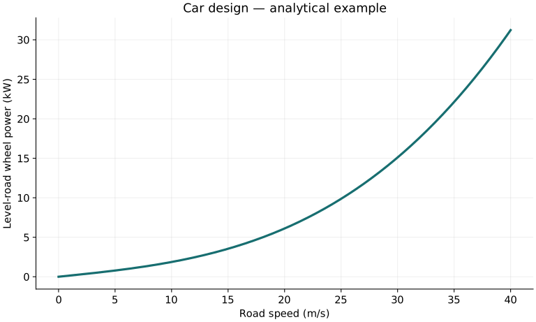
Twenty worked examples
Open a problem to see its defined inputs, assumptions, equation, numerical substitution, result, and interpretation. Values are illustrative analytical exercises.
Example 01. Aerodynamic drag
Definitions & inputs. ρ1.2,Cd.3,A2.2m²,V30m/s.
Choose the governing model and isolate the requested quantity.
Insert the stated inputs in consistent units or the explicitly defined normalized units.
Evaluate the expression; the result uses the units shown.
Interpretation. No wind.
↑ Return to definitions and contentsExample 02. Rolling resistance
Definitions & inputs. Crr.01,m1500kg,g9.81.
Choose the governing model and isolate the requested quantity.
Insert the stated inputs in consistent units or the explicitly defined normalized units.
Evaluate the expression; the result uses the units shown.
Interpretation. Level road.
↑ Return to definitions and contentsExample 03. Cruise wheel power
Definitions & inputs. Drag356.4N,rolling147.15N,V30m/s.
Choose the governing model and isolate the requested quantity.
Insert the stated inputs in consistent units or the explicitly defined normalized units.
Evaluate the expression; the result uses the units shown.
Interpretation. Excludes accessories and drivetrain loss.
↑ Return to definitions and contentsExample 04. Grade force
Definitions & inputs. m1500kg,sinθ.05.
Choose the governing model and isolate the requested quantity.
Insert the stated inputs in consistent units or the explicitly defined normalized units.
Evaluate the expression; the result uses the units shown.
Interpretation. Stated sinθ,not exact percent grade conversion.
↑ Return to definitions and contentsExample 05. Acceleration force
Definitions & inputs. m1500kg,a2m/s².
Choose the governing model and isolate the requested quantity.
Insert the stated inputs in consistent units or the explicitly defined normalized units.
Evaluate the expression; the result uses the units shown.
Interpretation. Add road loads for required wheel force.
↑ Return to definitions and contentsExample 06. Wheel torque
Definitions & inputs. F3000N,r.3m.
Choose the governing model and isolate the requested quantity.
Insert the stated inputs in consistent units or the explicitly defined normalized units.
Evaluate the expression; the result uses the units shown.
Interpretation. Total drive wheel torque.
↑ Return to definitions and contentsExample 07. Motor torque
Definitions & inputs. Tw900Nm,i9,η.95.
Choose the governing model and isolate the requested quantity.
Insert the stated inputs in consistent units or the explicitly defined normalized units.
Evaluate the expression; the result uses the units shown.
Interpretation. Fixed gearing.
↑ Return to definitions and contentsExample 08. Motor speed
Definitions & inputs. V30m/s,r.3m,i9.
Choose the governing model and isolate the requested quantity.
Insert the stated inputs in consistent units or the explicitly defined normalized units.
Evaluate the expression; the result uses the units shown.
Interpretation. Slip neglected.
↑ Return to definitions and contentsExample 09. Shaft rpm
Definitions & inputs. ω900rad/s.
Choose the governing model and isolate the requested quantity.
Insert the stated inputs in consistent units or the explicitly defined normalized units.
Evaluate the expression; the result uses the units shown.
Interpretation. Angular-speed conversion.
↑ Return to definitions and contentsExample 10. Adhesion force
Definitions & inputs. μ.8,Ndriven7000N.
Choose the governing model and isolate the requested quantity.
Insert the stated inputs in consistent units or the explicitly defined normalized units.
Evaluate the expression; the result uses the units shown.
Interpretation. Ideal friction ceiling.
↑ Return to definitions and contentsExample 11. Braking distance
Definitions & inputs. V20m/s,a7m/s².
Choose the governing model and isolate the requested quantity.
Insert the stated inputs in consistent units or the explicitly defined normalized units.
Evaluate the expression; the result uses the units shown.
Interpretation. Braking only,excludes reaction.
↑ Return to definitions and contentsExample 12. Reaction distance
Definitions & inputs. V20m/s,t1s.
Choose the governing model and isolate the requested quantity.
Insert the stated inputs in consistent units or the explicitly defined normalized units.
Evaluate the expression; the result uses the units shown.
Interpretation. Add to braking distance for this assumed reaction time.
↑ Return to definitions and contentsExample 13. Cornering acceleration
Definitions & inputs. V15m/s,R50m.
Choose the governing model and isolate the requested quantity.
Insert the stated inputs in consistent units or the explicitly defined normalized units.
Evaluate the expression; the result uses the units shown.
Interpretation. Steady turn.
↑ Return to definitions and contentsExample 14. Low-speed steering
Definitions & inputs. L2.7m,R50m.
Choose the governing model and isolate the requested quantity.
Insert the stated inputs in consistent units or the explicitly defined normalized units.
Evaluate the expression; the result uses the units shown.
Interpretation. Bicycle approximation.
↑ Return to definitions and contentsExample 15. Load transfer
Definitions & inputs. m1500,a7,h.5,L2.7SI.
Choose the governing model and isolate the requested quantity.
Insert the stated inputs in consistent units or the explicitly defined normalized units.
Evaluate the expression; the result uses the units shown.
Interpretation. Axle load increment on level road.
↑ Return to definitions and contentsExample 16. Quarter-car frequency
Definitions & inputs. k20000N/m,m350kg.
Choose the governing model and isolate the requested quantity.
Insert the stated inputs in consistent units or the explicitly defined normalized units.
Evaluate the expression; the result uses the units shown.
Interpretation. Single ride mode.
↑ Return to definitions and contentsExample 17. Critical damping
Definitions & inputs. Samek,m.
Choose the governing model and isolate the requested quantity.
Insert the stated inputs in consistent units or the explicitly defined normalized units.
Evaluate the expression; the result uses the units shown.
Interpretation. Critical damping coefficient.
↑ Return to definitions and contentsExample 18. Damping ratio
Definitions & inputs. c1500,k20000,m350SI.
Choose the governing model and isolate the requested quantity.
Insert the stated inputs in consistent units or the explicitly defined normalized units.
Evaluate the expression; the result uses the units shown.
Interpretation. Linear ride model.
↑ Return to definitions and contentsExample 19. Stopping energy
Definitions & inputs. m1500kg,V20m/s.
Choose the governing model and isolate the requested quantity.
Insert the stated inputs in consistent units or the explicitly defined normalized units.
Evaluate the expression; the result uses the units shown.
Interpretation. Rotating inertia omitted.
↑ Return to definitions and contentsExample 20. Cruise energy per distance
Definitions & inputs. Constant wheel power15kW,speed100km/h.
Choose the governing model and isolate the requested quantity.
Insert the stated inputs in consistent units or the explicitly defined normalized units.
Evaluate the expression; the result uses the units shown.
Interpretation. Wheel energy only.
↑ Return to definitions and contentsSymbols and units
Each derivation and problem defines its own symbols and inputs. Symbols may be reused with different meanings in other subjects. Keep units consistent, retain sufficient precision during calculation, and apply the stated validity limits.