PHYSICS / ENGINEERING / COMPUTING
Control theory models
Move from differential equations to feedback, transient response, frequency response and state-space reasoning, with twenty solved examples.
Matter pathway: atom → solid → liquid → gas → plasma. Quantum mechanics and quantum field theory provide foundations across the pathway; they are not additional phases. This is a connected modeling route, not a universal heating curve. Actual phases depend on pressure, composition, and kinetics.
1. Dynamics and transfer functions
Definitions & inputs. u input,y output,τ time constant,K static gain,s Laplace variable.
A first-order balance describes one dominant storage mode.
Laplace transformation turns differentiation into multiplication by s.
Invert the unit-step response with zero initial output.
Interpretation. Initial-state responses must be added when the system does not start at rest.
↑ Return to definitions and contents2. Negative feedback
Definitions & inputs. r reference,e error,C controller,G plant,T closed-loop transfer.
Substitute the controller and plant relations into the feedback equation.
Solve for output and error; T+S=1.
Proportional, integral and derivative actions shape the loop.
Interpretation. Ideal differentiation amplifies high-frequency noise and normally needs a filter.
↑ Return to definitions and contents3. Poles and transient response
Definitions & inputs. ζ damping ratio,ωn natural frequency,ωd damped frequency.
Normalize a second-order characteristic polynomial.
Complex poles set the oscillation rate and first response peak.
Exponential decay gives overshoot and a common approximate two-percent settling estimate.
Interpretation. Extra poles, zeros, delays and nonlinearities can invalidate these estimates.
↑ Return to definitions and contents4. Frequency and state space
Definitions & inputs. x state,A dynamics matrix,B input matrix,C output matrix,Ts sample period.
Separate internal memory from measured output.
Integrate the held-input state equation exactly.
Measure phase distance from negative feedback becoming positive at gain crossover.
Interpretation. Margin interpretation needs the complete loop and treatment of unstable open-loop poles.
↑ Return to definitions and contentsGraphical worked example
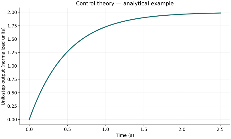
Twenty worked examples
Open a problem to see its defined inputs, assumptions, equation, numerical substitution, result, and interpretation. Values are illustrative analytical exercises.
Example 01. First-order pole
Definitions & inputs. τ=.5 s,K=2.
Choose the governing model and isolate the requested quantity.
Insert the stated inputs in consistent units or the explicitly defined normalized units.
Evaluate the expression; the result uses the units shown.
Interpretation. A negative real pole gives exponential decay.
↑ Return to definitions and contentsExample 02. Step after one time constant
Definitions & inputs. K=2,unit step,t=τ.
Choose the governing model and isolate the requested quantity.
Insert the stated inputs in consistent units or the explicitly defined normalized units.
Evaluate the expression; the result uses the units shown.
Interpretation. Final output is 2 in compatible output units.
↑ Return to definitions and contentsExample 03. First-order 95% rise
Definitions & inputs. τ=.5 s,target y/K=.95.
Choose the governing model and isolate the requested quantity.
Insert the stated inputs in consistent units or the explicitly defined normalized units.
Evaluate the expression; the result uses the units shown.
Interpretation. This is time to 95%, not the 10–90% rise-time definition.
↑ Return to definitions and contentsExample 04. Closed-loop static gain
Definitions & inputs. Plant static gain 2,proportional gain 3,unity negative feedback.
Choose the governing model and isolate the requested quantity.
Insert the stated inputs in consistent units or the explicitly defined normalized units.
Evaluate the expression; the result uses the units shown.
Interpretation. Finite proportional gain leaves steady tracking error.
↑ Return to definitions and contentsExample 05. Unit-step error
Definitions & inputs. Same static loop gain 6,stable type-0 loop.
Choose the governing model and isolate the requested quantity.
Insert the stated inputs in consistent units or the explicitly defined normalized units.
Evaluate the expression; the result uses the units shown.
Interpretation. The final-value theorem requires a stable closed-loop response.
↑ Return to definitions and contentsExample 06. Sensitivity magnitude at DC
Definitions & inputs. Real DC loop gain 9.
Choose the governing model and isolate the requested quantity.
Insert the stated inputs in consistent units or the explicitly defined normalized units.
Evaluate the expression; the result uses the units shown.
Interpretation. Sensitivity reduction at DC may be offset at other frequencies.
↑ Return to definitions and contentsExample 07. Closed-loop time constant
Definitions & inputs. G=2/(.5s+1),Kp=3,unity feedback.
Choose the governing model and isolate the requested quantity.
Insert the stated inputs in consistent units or the explicitly defined normalized units.
Evaluate the expression; the result uses the units shown.
Interpretation. The output gain also changes; speed alone is not the whole response.
↑ Return to definitions and contentsExample 08. Damped natural frequency
Definitions & inputs. ωn=10 rad/s,ζ=.6.
Choose the governing model and isolate the requested quantity.
Insert the stated inputs in consistent units or the explicitly defined normalized units.
Evaluate the expression; the result uses the units shown.
Interpretation. This is the oscillatory part of the pole pair.
↑ Return to definitions and contentsExample 09. Second-order peak time
Definitions & inputs. ωd=8 rad/s.
Choose the governing model and isolate the requested quantity.
Insert the stated inputs in consistent units or the explicitly defined normalized units.
Evaluate the expression; the result uses the units shown.
Interpretation. Standard zero-free second-order unit-step response is assumed.
↑ Return to definitions and contentsExample 10. Second-order overshoot
Definitions & inputs. ζ=.6.
Choose the governing model and isolate the requested quantity.
Insert the stated inputs in consistent units or the explicitly defined normalized units.
Evaluate the expression; the result uses the units shown.
Interpretation. Multiply by 100 to obtain percent overshoot.
↑ Return to definitions and contentsExample 11. Approximate settling time
Definitions & inputs. ζ=.6,ωn=10 rad/s,two-percent criterion.
Choose the governing model and isolate the requested quantity.
Insert the stated inputs in consistent units or the explicitly defined normalized units.
Evaluate the expression; the result uses the units shown.
Interpretation. This is a common envelope estimate, not an exact last crossing.
↑ Return to definitions and contentsExample 12. First-order gain at corner
Definitions & inputs. G=1/(τs+1),ωτ=1.
Choose the governing model and isolate the requested quantity.
Insert the stated inputs in consistent units or the explicitly defined normalized units.
Evaluate the expression; the result uses the units shown.
Interpretation. The magnitude is approximately −3.01 dB.
↑ Return to definitions and contentsExample 13. First-order phase at corner
Definitions & inputs. ωτ=1.
Choose the governing model and isolate the requested quantity.
Insert the stated inputs in consistent units or the explicitly defined normalized units.
Evaluate the expression; the result uses the units shown.
Interpretation. The phase approaches −90° only at much higher frequency.
↑ Return to definitions and contentsExample 14. Phase margin
Definitions & inputs. Loop phase −135° at a unit-magnitude crossover.
Choose the governing model and isolate the requested quantity.
Insert the stated inputs in consistent units or the explicitly defined normalized units.
Evaluate the expression; the result uses the units shown.
Interpretation. Other crossovers and unstable open-loop poles must also be considered.
↑ Return to definitions and contentsExample 15. Delay-induced phase
Definitions & inputs. Added delay .02 s at ω=10 rad/s.
Choose the governing model and isolate the requested quantity.
Insert the stated inputs in consistent units or the explicitly defined normalized units.
Evaluate the expression; the result uses the units shown.
Interpretation. Pure delay does not change magnitude but consumes phase margin.
↑ Return to definitions and contentsExample 16. Integrator accumulation
Definitions & inputs. Ki=2 s⁻¹,constant error .1 for 3 s,initial integral zero.
Choose the governing model and isolate the requested quantity.
Insert the stated inputs in consistent units or the explicitly defined normalized units.
Evaluate the expression; the result uses the units shown.
Interpretation. Saturation needs anti-windup treatment.
↑ Return to definitions and contentsExample 17. Derivative command
Definitions & inputs. Kd=.5 s,error slope .2/s.
Choose the governing model and isolate the requested quantity.
Insert the stated inputs in consistent units or the explicitly defined normalized units.
Evaluate the expression; the result uses the units shown.
Interpretation. Real derivative action is filtered to limit noise amplification.
↑ Return to definitions and contentsExample 18. Exact sampled decay
Definitions & inputs. Continuous dx/dt=−2x,Ts=.1 s.
Choose the governing model and isolate the requested quantity.
Insert the stated inputs in consistent units or the explicitly defined normalized units.
Evaluate the expression; the result uses the units shown.
Interpretation. Repeated multiplication reproduces exact sample values for the unforced model.
↑ Return to definitions and contentsExample 19. Euler stability limit
Definitions & inputs. dx/dt=−2x,forward Euler.
Choose the governing model and isolate the requested quantity.
Insert the stated inputs in consistent units or the explicitly defined normalized units.
Evaluate the expression; the result uses the units shown.
Interpretation. The upper endpoint itself is not asymptotically stable; accuracy usually needs much smaller steps.
↑ Return to definitions and contentsExample 20. Scalar state-feedback pole
Definitions & inputs. dx/dt=−x+u,u=−3x.
Choose the governing model and isolate the requested quantity.
Insert the stated inputs in consistent units or the explicitly defined normalized units.
Evaluate the expression; the result uses the units shown.
Interpretation. State measurement and actuator authority are assumed.
↑ Return to definitions and contentsSymbols and units
Each derivation and problem defines its own symbols and inputs. Symbols may be reused with different meanings in other subjects. Keep units consistent, retain sufficient precision during calculation, and apply the stated validity limits.