PHYSICS / ENGINEERING / COMPUTING
Computer chip design models
Connect logic, timing, power, interconnect, floorplanning, and yield through twenty worked implementation estimates.
Matter pathway: atom → solid → liquid → gas → plasma. Quantum mechanics and quantum field theory provide foundations across the pathway; they are not additional phases. This is a connected modeling route, not a universal heating curve. Actual phases depend on pressure, composition, and kinetics.
1. From logic to implementation
Definitions & inputs. RTL describes behavior; gates implement Boolean functions; N denotes counts, not physical transistor area.
Boolean logic establishes functionality before physical implementation.
n binary storage bits represent this many bit patterns.
Each stage refines timing, physical connectivity, and manufacturing constraints.
Interpretation. Correct logic alone does not guarantee a manufacturable or timing-clean chip.
↑ Return to definitions and contents2. Setup, hold, and path delay
Definitions & inputs. tcq clock-to-Q delay, tcomb combinational path delay, tsetup setup time, u clock uncertainty.
Latest data arrival must precede the next capture edge by setup time.
Positive slack means this modeled path meets setup.
Earliest data must not disturb the capture register’s hold window.
Interpretation. Increasing the clock period does not directly fix a hold violation.
↑ Return to definitions and contents3. Switching energy and interconnect
Definitions & inputs. α is expected 0→1 transitions per clock, C switched capacitance, V supply, f frequency, Ileak leakage current.
Each complete charge event draws CV² from the supply; half is stored and later dissipated.
Leakage and first-order wire/load delay use different models.
Geometry and current set resistive voltage loss.
Interpretation. Parasitic extraction and activity characterization replace these estimates in signoff.
↑ Return to definitions and contents4. Area, thermal budgets, and manufacturing yield
Definitions & inputs. Acell is total cell area, U utilization, D0 defect density, θJA package thermal resistance.
Reserve space for routing and physical optimization.
A Poisson no-defect probability estimates yield for random area defects.
Steady thermal resistance maps power to a junction temperature estimate.
Interpretation. Utilization, yield, and thermal margin are separate constraints; none replaces full design-rule and reliability checks.
↑ Return to definitions and contentsGraphical worked example
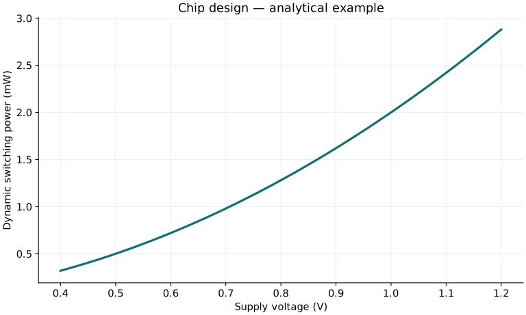
Twenty worked examples
Open a problem to see its defined inputs, assumptions, equation, numerical substitution, result, and interpretation. Values are illustrative analytical exercises.
Example 01. Register state count
Definitions & inputs. n=8 bits.
Choose the governing model and isolate the requested quantity.
Insert the stated inputs in consistent units or the explicitly defined normalized units.
Evaluate the expression; the result uses the units shown.
Interpretation. This is representable states, not clock cycles.
↑ Return to definitions and contentsExample 02. Memory bit count
Definitions & inputs. 1024 words, 32 bits per word.
Choose the governing model and isolate the requested quantity.
Insert the stated inputs in consistent units or the explicitly defined normalized units.
Evaluate the expression; the result uses the units shown.
Interpretation. The raw payload is 4 KiB before ECC and addressing overhead.
↑ Return to definitions and contentsExample 03. Setup-limited period
Definitions & inputs. tcq=80 ps, combinational delay 600 ps, setup 70 ps, uncertainty 50 ps.
Choose the governing model and isolate the requested quantity.
Insert the stated inputs in consistent units or the explicitly defined normalized units.
Evaluate the expression; the result uses the units shown.
Interpretation. Corresponding ideal maximum clock is 1.25 GHz for this path.
↑ Return to definitions and contentsExample 04. Maximum frequency
Definitions & inputs. Tmin=800 ps.
Choose the governing model and isolate the requested quantity.
Insert the stated inputs in consistent units or the explicitly defined normalized units.
Evaluate the expression; the result uses the units shown.
Interpretation. Other paths or corners can lower the design limit.
↑ Return to definitions and contentsExample 05. Setup slack
Definitions & inputs. Clock period 1000 ps, modeled required path budget 800 ps.
Choose the governing model and isolate the requested quantity.
Insert the stated inputs in consistent units or the explicitly defined normalized units.
Evaluate the expression; the result uses the units shown.
Interpretation. Positive slack is remaining setup margin.
↑ Return to definitions and contentsExample 06. Hold slack
Definitions & inputs. tcq,min=30 ps, tcomb,min=20 ps, thold=40 ps, uncertainty=5 ps.
Choose the governing model and isolate the requested quantity.
Insert the stated inputs in consistent units or the explicitly defined normalized units.
Evaluate the expression; the result uses the units shown.
Interpretation. Only five picoseconds of hold margin remain.
↑ Return to definitions and contentsExample 07. Dynamic power
Definitions & inputs. α=0.2, C=10 pF, V=1 V, f=1 GHz.
Choose the governing model and isolate the requested quantity.
Insert the stated inputs in consistent units or the explicitly defined normalized units.
Evaluate the expression; the result uses the units shown.
Interpretation. Activity counts 0→1 charge events per clock.
↑ Return to definitions and contentsExample 08. Voltage-scaling power ratio
Definitions & inputs. Supply changes 1.0 V to 0.8 V, other factors fixed.
Choose the governing model and isolate the requested quantity.
Insert the stated inputs in consistent units or the explicitly defined normalized units.
Evaluate the expression; the result uses the units shown.
Interpretation. This alone predicts 36% less dynamic power; timing may worsen.
↑ Return to definitions and contentsExample 09. Leakage power
Definitions & inputs. V=0.8 V, aggregate leakage 2 mA.
Choose the governing model and isolate the requested quantity.
Insert the stated inputs in consistent units or the explicitly defined normalized units.
Evaluate the expression; the result uses the units shown.
Interpretation. Leakage can vary strongly with temperature and process.
↑ Return to definitions and contentsExample 10. Charge-event energy
Definitions & inputs. C=20 fF, V=0.8 V.
Choose the governing model and isolate the requested quantity.
Insert the stated inputs in consistent units or the explicitly defined normalized units.
Evaluate the expression; the result uses the units shown.
Interpretation. This is supply energy for charging, not the stored half-CV² energy.
↑ Return to definitions and contentsExample 11. Lumped interconnect delay
Definitions & inputs. R=1 kΩ, C=20 fF.
Choose the governing model and isolate the requested quantity.
Insert the stated inputs in consistent units or the explicitly defined normalized units.
Evaluate the expression; the result uses the units shown.
Interpretation. This is the 50% delay of a single-pole step approximation.
↑ Return to definitions and contentsExample 12. Wire resistance
Definitions & inputs. ρ=2×10⁻⁸ Ωm, length 1 mm, cross section 1 µm².
Choose the governing model and isolate the requested quantity.
Insert the stated inputs in consistent units or the explicitly defined normalized units.
Evaluate the expression; the result uses the units shown.
Interpretation. Narrower or longer wires raise resistance.
↑ Return to definitions and contentsExample 13. Supply IR drop
Definitions & inputs. Rail current 20 mA, effective path resistance 0.5 Ω.
Choose the governing model and isolate the requested quantity.
Insert the stated inputs in consistent units or the explicitly defined normalized units.
Evaluate the expression; the result uses the units shown.
Interpretation. Ten millivolts is a DC estimate; switching adds transient effects.
↑ Return to definitions and contentsExample 14. Core area from utilization
Definitions & inputs. Cell area 2 mm², target utilization U=0.6.
Choose the governing model and isolate the requested quantity.
Insert the stated inputs in consistent units or the explicitly defined normalized units.
Evaluate the expression; the result uses the units shown.
Interpretation. Routing and macros can require a different practical footprint.
↑ Return to definitions and contentsExample 15. Square core dimension
Definitions & inputs. Core area 4 mm².
Choose the governing model and isolate the requested quantity.
Insert the stated inputs in consistent units or the explicitly defined normalized units.
Evaluate the expression; the result uses the units shown.
Interpretation. Aspect ratio changes dimensions at fixed area.
↑ Return to definitions and contentsExample 16. Poisson defect yield
Definitions & inputs. D0=0.1 defects/cm², die area A=1 cm².
Choose the governing model and isolate the requested quantity.
Insert the stated inputs in consistent units or the explicitly defined normalized units.
Evaluate the expression; the result uses the units shown.
Interpretation. This predicts random-area defect-free yield only.
↑ Return to definitions and contentsExample 17. Expected good dies
Definitions & inputs. Gross dies=500, yield=0.9.
Choose the governing model and isolate the requested quantity.
Insert the stated inputs in consistent units or the explicitly defined normalized units.
Evaluate the expression; the result uses the units shown.
Interpretation. Expected count is not a guaranteed lot outcome.
↑ Return to definitions and contentsExample 18. Junction temperature
Definitions & inputs. Ta=25°C, θJA=20 K/W, P=2 W.
Choose the governing model and isolate the requested quantity.
Insert the stated inputs in consistent units or the explicitly defined normalized units.
Evaluate the expression; the result uses the units shown.
Interpretation. Package and board conditions determine θJA.
↑ Return to definitions and contentsExample 19. Amdahl speedup
Definitions & inputs. Fraction accelerated f=0.8, that block becomes 4× faster.
Choose the governing model and isolate the requested quantity.
Insert the stated inputs in consistent units or the explicitly defined normalized units.
Evaluate the expression; the result uses the units shown.
Interpretation. Speeding one block does not multiply whole-system speed by four.
↑ Return to definitions and contentsExample 20. Pipeline throughput
Definitions & inputs. One result each clock at f=500 MHz after filling.
Choose the governing model and isolate the requested quantity.
Insert the stated inputs in consistent units or the explicitly defined normalized units.
Evaluate the expression; the result uses the units shown.
Interpretation. Latency can still be many cycles; initiation interval is one.
↑ Return to definitions and contentsSymbols and units
Each derivation and problem defines its own symbols and inputs. Symbols may be reused with different meanings in other subjects. Keep units consistent, retain sufficient precision during calculation, and apply the stated validity limits.