PHYSICS / ENGINEERING / COMPUTING
Uncertainty quantification in measurement and models
Build uncertainty budgets, propagate correlated inputs, compare Monte Carlo and linear methods, and separate numerical error from model discrepancy.
Matter pathway: atom → solid → liquid → gas → plasma. Quantum mechanics and quantum field theory provide foundations across the pathway; they are not additional phases. This is a connected modeling route, not a universal heating curve. Actual phases depend on pressure, composition, and kinetics.
1. Measurement equation and sensitivity
Definitions & inputs. y=f(x),ui standard uncertainties,C covariance matrix,J gradient at input estimates.
Taylor-expand about nominal input values.
Propagate both variance and covariance.
A shared calibration error can prevent averaging benefits.
Interpretation. Standard uncertainty is not an error bound. Correct known bias where possible and retain uncertainty in that correction.
↑ Return to definitions and contents2. Nonlinear propagation and Monte Carlo
Definitions & inputs. X input random vector,Y=f(X),Ns draws,smc sampling standard error.
Simulate the measurement or physical model with input draws.
Estimate output moments and their simulation error for independent draws.
Quantiles describe asymmetric coverage intervals when a symmetric linear approximation is poor.
Interpretation. Check convergence of tails separately; rare-event probabilities can need importance sampling. Correlated MCMC samples need effective sample-size analysis.
↑ Return to definitions and contents3. Sensitivity and surrogate models
Definitions & inputs. Vi variance attributable to input i,V output variance,STi total-effect So bol index.
Orthogonal functional ANOVA separates main effects and interactions.
First-order and total-effect indices answer different sensitivity questions.
Polynomial chaos is one surrogate option; Gaussian processes and response surfaces have different assumptions.
Interpretation. Local derivatives, global variance shares and causal effects are not interchangeable. Validate surrogates where decisions depend on their accuracy.
↑ Return to definitions and contents4. Calibration, discrepancy and verification
Definitions & inputs. d observations,f(θ) simulator,δ discrepancy,ε measurement noise,h mesh size,p observed convergence order.
Separate parameter uncertainty, missing physics and measurement error.
Bayesian calibration must include the assumptions defining the likelihood and discrepancy.
Extrapolate a leading discretization term when the convergence model applies.
Interpretation. Calibration is not validation; numerical convergence is not physical accuracy. Report input distributions, correlations, solver error, discrepancy assumptions, coverage meaning and sensitivity results.
↑ Return to definitions and contentsGraphical worked example
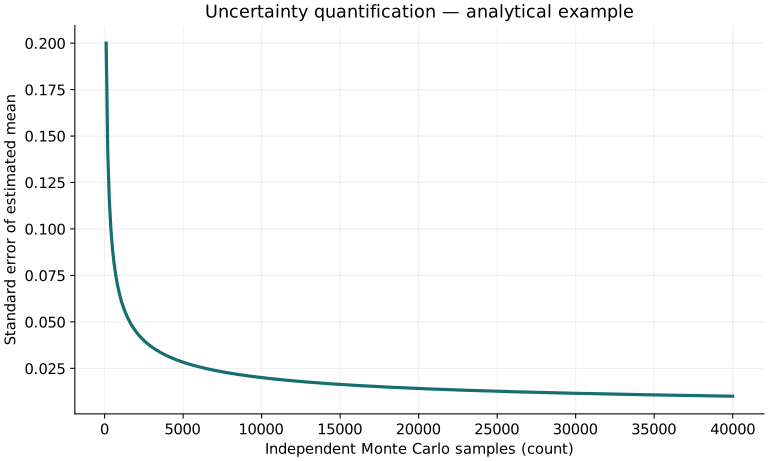
Twenty worked examples
Open a problem to see its defined inputs, assumptions, equation, numerical substitution, result, and interpretation. Values are illustrative analytical exercises.
Example 01. Independent sum uncertainty
Definitions & inputs. u1.3,u2.4.
Choose the governing model and isolate the requested quantity.
Insert the stated inputs in consistent units or the explicitly defined normalized units.
Evaluate the expression; the result uses the units shown.
Interpretation. Same input units.
↑ Return to definitions and contentsExample 02. Correlated sum
Definitions & inputs. u1.3,u2.4,ρ.5.
Choose the governing model and isolate the requested quantity.
Insert the stated inputs in consistent units or the explicitly defined normalized units.
Evaluate the expression; the result uses the units shown.
Interpretation. Positive correlation increases uncertainty.
↑ Return to definitions and contentsExample 03. Difference with common bias
Definitions & inputs. Equalu1=u2=.2,ρ1.
Choose the governing model and isolate the requested quantity.
Insert the stated inputs in consistent units or the explicitly defined normalized units.
Evaluate the expression; the result uses the units shown.
Interpretation. Perfect shared additive error cancels in this idealized difference.
↑ Return to definitions and contentsExample 04. Scale sensitivity
Definitions & inputs. y3x.
Choose the governing model and isolate the requested quantity.
Insert the stated inputs in consistent units or the explicitly defined normalized units.
Evaluate the expression; the result uses the units shown.
Interpretation. Coefficient units follow the model.
↑ Return to definitions and contentsExample 05. Scaled uncertainty
Definitions & inputs. y3x,ux.2.
Choose the governing model and isolate the requested quantity.
Insert the stated inputs in consistent units or the explicitly defined normalized units.
Evaluate the expression; the result uses the units shown.
Interpretation. Linear propagation exact.
↑ Return to definitions and contentsExample 06. Relative product uncertainty
Definitions & inputs. Independent relative uncertainties.02,.03.
Choose the governing model and isolate the requested quantity.
Insert the stated inputs in consistent units or the explicitly defined normalized units.
Evaluate the expression; the result uses the units shown.
Interpretation. First-order product law.
↑ Return to definitions and contentsExample 07. Area sensitivity
Definitions & inputs. Circle r2m.
Choose the governing model and isolate the requested quantity.
Insert the stated inputs in consistent units or the explicitly defined normalized units.
Evaluate the expression; the result uses the units shown.
Interpretation. Gradient ofπr².
↑ Return to definitions and contentsExample 08. Area uncertainty
Definitions & inputs. r2m,ur.01m.
Choose the governing model and isolate the requested quantity.
Insert the stated inputs in consistent units or the explicitly defined normalized units.
Evaluate the expression; the result uses the units shown.
Interpretation. Small radius uncertainty.
↑ Return to definitions and contentsExample 09. Uniform tolerance standard uncertainty
Definitions & inputs. Uniform error±.1mm.
Choose the governing model and isolate the requested quantity.
Insert the stated inputs in consistent units or the explicitly defined normalized units.
Evaluate the expression; the result uses the units shown.
Interpretation. Uniform distribution assumption explicit.
↑ Return to definitions and contentsExample 10. Quantization uncertainty
Definitions & inputs. Step.01V,uniform rounding.
Choose the governing model and isolate the requested quantity.
Insert the stated inputs in consistent units or the explicitly defined normalized units.
Evaluate the expression; the result uses the units shown.
Interpretation. Not all ADC errors are quantization.
↑ Return to definitions and contentsExample 11. Expanded uncertainty
Definitions & inputs. u.5,k2.
Choose the governing model and isolate the requested quantity.
Insert the stated inputs in consistent units or the explicitly defined normalized units.
Evaluate the expression; the result uses the units shown.
Interpretation. Approximately95percent only under appropriate coverage assumptions.
↑ Return to definitions and contentsExample 12. Monte Carlo mean SE
Definitions & inputs. Output standard deviation2,N10000independent draws.
Choose the governing model and isolate the requested quantity.
Insert the stated inputs in consistent units or the explicitly defined normalized units.
Evaluate the expression; the result uses the units shown.
Interpretation. Simulation error,not physical output spread.
↑ Return to definitions and contentsExample 13. Draw count for target SE
Definitions & inputs. s2,target.01.
Choose the governing model and isolate the requested quantity.
Insert the stated inputs in consistent units or the explicitly defined normalized units.
Evaluate the expression; the result uses the units shown.
Interpretation. Estimated finite variance assumption.
↑ Return to definitions and contentsExample 14. Bernoulli probability SE
Definitions & inputs. p.01,N10000.
Choose the governing model and isolate the requested quantity.
Insert the stated inputs in consistent units or the explicitly defined normalized units.
Evaluate the expression; the result uses the units shown.
Interpretation. Tail estimation can be relatively noisy.
↑ Return to definitions and contentsExample 15. Zero-event upper bound
Definitions & inputs. Zero events,N1000,one-sided95percent.
Choose the governing model and isolate the requested quantity.
Insert the stated inputs in consistent units or the explicitly defined normalized units.
Evaluate the expression; the result uses the units shown.
Interpretation. Exact binomial upper bound under independence.
↑ Return to definitions and contentsExample 16. Nonlinear mean correction
Definitions & inputs. Xmean2,variance.25,Y=X².
Choose the governing model and isolate the requested quantity.
Insert the stated inputs in consistent units or the explicitly defined normalized units.
Evaluate the expression; the result uses the units shown.
Interpretation. Plugging the mean into f would miss.25.
↑ Return to definitions and contentsExample 17. First-order Sobol share
Definitions & inputs. Vi2,totalV5.
Choose the governing model and isolate the requested quantity.
Insert the stated inputs in consistent units or the explicitly defined normalized units.
Evaluate the expression; the result uses the units shown.
Interpretation. Independent-input decomposition.
↑ Return to definitions and contentsExample 18. Total-effect index
Definitions & inputs. Var conditional mean3,total5.
Choose the governing model and isolate the requested quantity.
Insert the stated inputs in consistent units or the explicitly defined normalized units.
Evaluate the expression; the result uses the units shown.
Interpretation. Includes interactions with that input.
↑ Return to definitions and contentsExample 19. Richardson extrapolation
Definitions & inputs. fh1.04,fh2=1.01,p2.
Choose the governing model and isolate the requested quantity.
Insert the stated inputs in consistent units or the explicitly defined normalized units.
Evaluate the expression; the result uses the units shown.
Interpretation. Asymptotic leading error assumed.
↑ Return to definitions and contentsExample 20. Independent discrepancy combination
Definitions & inputs. Measurement u.2,model discrepancy sd.5.
Choose the governing model and isolate the requested quantity.
Insert the stated inputs in consistent units or the explicitly defined normalized units.
Evaluate the expression; the result uses the units shown.
Interpretation. Assumed zero mean independent discrepancy;not universal.
↑ Return to definitions and contentsSymbols and units
Each derivation and problem defines its own symbols and inputs. Symbols may be reused with different meanings in other subjects. Keep units consistent, retain sufficient precision during calculation, and apply the stated validity limits.