PHYSICS / ENGINEERING / COMPUTING
Embedded software and real-time systems
Derive timing, scheduling, sampling, buffering, fixed-point, and energy budgets, with twenty worked calculations.
Matter pathway: atom → solid → liquid → gas → plasma. Quantum mechanics and quantum field theory provide foundations across the pathway; they are not additional phases. This is a connected modeling route, not a universal heating curve. Actual phases depend on pressure, composition, and kinetics.
1. Clocks and execution
Definitions & inputs. fclk clock frequency, Ncycles executed cycles, C execution time, T task period.
Convert clock counts into elapsed time.
Add each periodic task’s required processor fraction.
This sufficient rate-monotonic bound assumes independent preemptible periodic tasks with deadlines equal to periods.
Interpretation. Exceeding the bound does not prove failure; use response-time analysis.
↑ Return to definitions and contents2. Response time and deadlines
Definitions & inputs. Ci execution, Bi blocking, Ti period, hp(i) higher-priority tasks, Ri response time.
Start with the task’s own demand plus blocking.
Count interfering releases within the tentative response window.
Stop at a fixed point or a missed deadline.
Interpretation. Interrupt service and context overhead must be included consistently.
↑ Return to definitions and contents3. Data movement and representation
Definitions & inputs. fs sample rate, b bits/sample, Δ quantizer step, x represented value.
Sampling defines the stream rate; integrate over a consumer pause for buffer bytes.
Divide the input span among N-bit bins and round to the nearest bin.
Fixed-point integer q represents a physical value with F fractional bits.
Interpretation. Guard against endpoint clipping, rounding conventions, and arithmetic overflow.
↑ Return to definitions and contents4. Energy and duty cycles
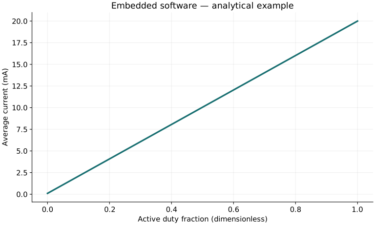
Definitions & inputs. Da active fraction, Ia and Is active/sleep currents, V supply voltage.
Time-weight the mode currents.
Integrate approximately constant power over the observation interval.
Divide usable capacity by average current using compatible hour units.
Interpretation. Radio bursts, self-discharge, voltage conversion, and wakeup latency can dominate.
↑ Return to definitions and contentsGraphical worked example
Twenty worked examples
Open a problem to see its defined inputs, assumptions, equation, numerical substitution, result, and interpretation. Values are illustrative analytical exercises.
Example 01. Clock tick
Definitions & inputs. Clock 48 MHz.
Choose the governing model and isolate the requested quantity.
Insert the stated inputs in consistent units or the explicitly defined normalized units.
Evaluate the expression; the result uses the units shown.
Interpretation. A clock tick is not necessarily a complete instruction.
↑ Return to definitions and contentsExample 02. Execution duration
Definitions & inputs. 2400 cycles at 48 MHz.
Choose the governing model and isolate the requested quantity.
Insert the stated inputs in consistent units or the explicitly defined normalized units.
Evaluate the expression; the result uses the units shown.
Interpretation. Memory stalls must already be included in the count.
↑ Return to definitions and contentsExample 03. Timer prescaler
Definitions & inputs. Source 48 MHz, desired timer tick 1 MHz.
Choose the governing model and isolate the requested quantity.
Insert the stated inputs in consistent units or the explicitly defined normalized units.
Evaluate the expression; the result uses the units shown.
Interpretation. Some timer registers encode P−1 rather than P.
↑ Return to definitions and contentsExample 04. Timer compare count
Definitions & inputs. Tick 1 μs, interval 2 ms.
Choose the governing model and isolate the requested quantity.
Insert the stated inputs in consistent units or the explicitly defined normalized units.
Evaluate the expression; the result uses the units shown.
Interpretation. Check whether the hardware counts inclusively from zero.
↑ Return to definitions and contentsExample 05. Task utilization
Definitions & inputs. C1=1 ms,T1=5 ms; C2=2 ms,T2=10 ms.
Choose the governing model and isolate the requested quantity.
Insert the stated inputs in consistent units or the explicitly defined normalized units.
Evaluate the expression; the result uses the units shown.
Interpretation. Forty percent excludes unlisted interrupt and kernel overhead.
↑ Return to definitions and contentsExample 06. Three-task sufficient bound
Definitions & inputs. n=3 independent periodic tasks under rate-monotonic scheduling.
Choose the governing model and isolate the requested quantity.
Insert the stated inputs in consistent units or the explicitly defined normalized units.
Evaluate the expression; the result uses the units shown.
Interpretation. This is sufficient, not necessary, under the stated ideal assumptions.
↑ Return to definitions and contentsExample 07. Low-priority response time
Definitions & inputs. Low task C=2 ms; high task C=1 ms,T=5 ms; B=0.
Choose the governing model and isolate the requested quantity.
Insert the stated inputs in consistent units or the explicitly defined normalized units.
Evaluate the expression; the result uses the units shown.
Interpretation. The fixed point is 3 ms; compare against the low task deadline.
↑ Return to definitions and contentsExample 08. Deadline slack
Definitions & inputs. Deadline 10 ms, worst-case response 7 ms.
Choose the governing model and isolate the requested quantity.
Insert the stated inputs in consistent units or the explicitly defined normalized units.
Evaluate the expression; the result uses the units shown.
Interpretation. Slack is meaningful only if the response bound is justified.
↑ Return to definitions and contentsExample 09. Interrupt overhead fraction
Definitions & inputs. 10000 interrupts/s, handler 2 μs each.
Choose the governing model and isolate the requested quantity.
Insert the stated inputs in consistent units or the explicitly defined normalized units.
Evaluate the expression; the result uses the units shown.
Interpretation. Entry, exit, and nesting costs must be included in handler time.
↑ Return to definitions and contentsExample 10. ADC voltage step
Definitions & inputs. 12-bit converter, full-scale span 3.3 V.
Choose the governing model and isolate the requested quantity.
Insert the stated inputs in consistent units or the explicitly defined normalized units.
Evaluate the expression; the result uses the units shown.
Interpretation. This is quantization step, not total accuracy.
↑ Return to definitions and contentsExample 11. Quantization error bound
Definitions & inputs. Step 0.8 mV; nearest rounding.
Choose the governing model and isolate the requested quantity.
Insert the stated inputs in consistent units or the explicitly defined normalized units.
Evaluate the expression; the result uses the units shown.
Interpretation. Noise and calibration error are additional effects.
↑ Return to definitions and contentsExample 12. Sampling data rate
Definitions & inputs. 1000 samples/s, 16 bits/sample.
Choose the governing model and isolate the requested quantity.
Insert the stated inputs in consistent units or the explicitly defined normalized units.
Evaluate the expression; the result uses the units shown.
Interpretation. Packet headers are not included.
↑ Return to definitions and contentsExample 13. Buffer for a pause
Definitions & inputs. Producer 2000 bytes/s; consumer unavailable 0.25 s; empty initial buffer.
Choose the governing model and isolate the requested quantity.
Insert the stated inputs in consistent units or the explicitly defined normalized units.
Evaluate the expression; the result uses the units shown.
Interpretation. Add margin for bursts and pre-existing queued data.
↑ Return to definitions and contentsExample 14. UART payload throughput
Definitions & inputs. 115200 bit/s, 8-N-1 framing: 10 transmitted bits per byte.
Choose the governing model and isolate the requested quantity.
Insert the stated inputs in consistent units or the explicitly defined normalized units.
Evaluate the expression; the result uses the units shown.
Interpretation. This excludes any protocol overhead or idle gaps.
↑ Return to definitions and contentsExample 15. SPI transfer duration
Definitions & inputs. 256 bytes at 8 Mbit/s; no gaps.
Choose the governing model and isolate the requested quantity.
Insert the stated inputs in consistent units or the explicitly defined normalized units.
Evaluate the expression; the result uses the units shown.
Interpretation. Chip-select setup and software latency add time.
↑ Return to definitions and contentsExample 16. Fixed-point decode
Definitions & inputs. Stored integer q=384, F=8 fractional bits.
Choose the governing model and isolate the requested quantity.
Insert the stated inputs in consistent units or the explicitly defined normalized units.
Evaluate the expression; the result uses the units shown.
Interpretation. Signed range depends on total word length.
↑ Return to definitions and contentsExample 17. Unsigned counter wrap
Definitions & inputs. 16-bit counter increments at 1 kHz.
Choose the governing model and isolate the requested quantity.
Insert the stated inputs in consistent units or the explicitly defined normalized units.
Evaluate the expression; the result uses the units shown.
Interpretation. Use modular subtraction only within a documented wrap interval.
↑ Return to definitions and contentsExample 18. Average current
Definitions & inputs. Active 20 mA for 10% time; sleep 0.1 mA.
Choose the governing model and isolate the requested quantity.
Insert the stated inputs in consistent units or the explicitly defined normalized units.
Evaluate the expression; the result uses the units shown.
Interpretation. Transition energy and radio peaks are omitted.
↑ Return to definitions and contentsExample 19. Ideal battery lifetime
Definitions & inputs. Usable capacity 1000 mAh, average current 2 mA.
Choose the governing model and isolate the requested quantity.
Insert the stated inputs in consistent units or the explicitly defined normalized units.
Evaluate the expression; the result uses the units shown.
Interpretation. The usable capacity has to reflect load and environment.
↑ Return to definitions and contentsExample 20. Watchdog timing margin
Definitions & inputs. Timeout 100 ms; maximum valid service gap 70 ms.
Choose the governing model and isolate the requested quantity.
Insert the stated inputs in consistent units or the explicitly defined normalized units.
Evaluate the expression; the result uses the units shown.
Interpretation. A watchdog detects missed service, not all forms of incorrect software execution.
↑ Return to definitions and contentsSymbols and units
Each derivation and problem defines its own symbols and inputs. Symbols may be reused with different meanings in other subjects. Keep units consistent, retain sufficient precision during calculation, and apply the stated validity limits.