PHYSICS / ENGINEERING / COMPUTING
Spallation calculation for satellite survivability
Connect stress-wave failure to spacecraft debris containment, test-based damage criteria and mission-level reliability.
Matter pathway: atom → solid → liquid → gas → plasma. Quantum mechanics and quantum field theory provide foundations across the pathway; they are not additional phases. This is a connected modeling route, not a universal heating curve. Actual phases depend on pressure, composition, and kinetics.
A satellite protection workflow
- Define the orbit, exposure duration and meteoroid/orbital-debris environment. NASA MEM and the orbital-debris environment are distinct inputs.
- Define failure for each component: detached rear-wall material, perforation, pressure leakage, electrical interruption or optical damage.
- Select a shield family and an experimentally supported ballistic-limit model within its stated material, velocity, angle and geometry range.
- Use dynamic material characterization and hydrocodes to investigate mechanisms; compare against witness plates, free-surface histories and recovered damage.
- Propagate uncertainty and inspect shared-fragment and common-cause failures before crediting redundancy.
Backing fabrics and catchers can absorb or redistribute debris, but their performance depends on construction, temperature, vacuum exposure, aging and mounting. Generic anti-spall marketing or a coating name is not a spacecraft qualification. This guide does not supply personnel-incapacitation coefficients or weapon-specific behind-armor models.
NASA impact physics and damage criteria · NASA meteoroid/debris shielding report · NASA meteoroid environment
1. Stress waves and tensile failure
Definitions & inputs. σ tensile-positive stress,ρ density,c wave speed,Z acoustic impedance,σsp measured dynamic spall strength.
Linear acoustics links particle-velocity change and stress amplitude.
A free surface reflects a compressive stress increment as a release/tensile increment; total traction at the surface remains zero.
Interacting release histories can place interior material in tension, initiating voiding or cracking.
Interpretation. A threshold alone does not predict detached mass or debris speed. Spall strength depends on microstructure, pulse duration, strain rate, temperature and measurement interpretation; not every free-surface reflection creates spall.
↑ Return to definitions and contents2. Damage models and hydrocode consistency
Definitions & inputs. D scalar damage0to1,σeff effective undamaged stress,εp plastic strain,α internal variables.
Scalar degradation shows how damage can reduce load-carrying capacity; tension/compression treatment needs a specified law.
Evolution must be calibrated to dynamic tests rather than inferred from static tensile strength.
A hydrocode evolves mass, momentum, energy and constitutive variables consistently.
Interpretation. Grady–Kipp families connect flaw populations, activation and fragmentation; Cochran–Banner-type models use tensile deformation and damage evolution. Names do not define a unique implementation. Mesh regularization, energy dissipation, EOS, strength and failure parameters must be documented and verified against tests.
↑ Return to definitions and contents3. Debris statistics and containment
Definitions & inputs. m fragment mass,N greater cumulative count,μ scale,n shape,N0 normalization,A exposed area,Φ environmental flux.
A stretched-exponential cumulative model can summarize fragment counts above a threshold.
μ is a scale, not generally the mean: for n1 it equals the mean; for n1/2 the mean is2μ.
An integrated directional environment may be simplified to this flux–area–time count only with consistent projected-area conventions.
Interpretation. Cone shapes, fragment velocity and damage cannot be transferred from unrelated armor tests or assigned a universal fraction of sound speed. Use witness plates, velocity diagnostics, recovered fragments and validated spacecraft-specific debris models.
↑ Return to definitions and contents4. From shield damage to mission survival
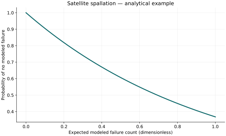
Definitions & inputs. λfail expected mission failure count,pf conditional component failure given an event,λevent expected impact count.
Integrate over size, velocity, direction, configuration and time using a calibrated failure criterion.
Poisson thinning produces a survival probability only for the defined event process.
A simplified bookkeeping example separates environment frequency from conditional damage.
Interpretation. Distinguish cratering, attached damage, detached spall, perforation, leakage and loss of function. Whipple and stuffed-Whipple shields, internal catchers, equipment placement and redundancy mitigate different outcomes; thermal blankets or coatings are not automatically qualified spall liners.
↑ Return to definitions and contentsGraphical worked example
Twenty worked examples
Open a problem to see its defined inputs, assumptions, equation, numerical substitution, result, and interpretation. Values are illustrative analytical exercises.
Example 01. One-way wave time
Definitions & inputs. L.01m,c5000m/s.
Choose the governing model and isolate the requested quantity.
Insert the stated inputs in consistent units or the explicitly defined normalized units.
Evaluate the expression; the result uses the units shown.
Interpretation. Elastic-wave timing only.
↑ Return to definitions and contentsExample 02. Round-trip time
Definitions & inputs. Same path.
Choose the governing model and isolate the requested quantity.
Insert the stated inputs in consistent units or the explicitly defined normalized units.
Evaluate the expression; the result uses the units shown.
Interpretation. Reflection timing benchmark.
↑ Return to definitions and contentsExample 03. Acoustic impedance
Definitions & inputs. ρ2700kg/m³,c5000m/s.
Choose the governing model and isolate the requested quantity.
Insert the stated inputs in consistent units or the explicitly defined normalized units.
Evaluate the expression; the result uses the units shown.
Interpretation. Illustrative material.
↑ Return to definitions and contentsExample 04. Free-surface stress reflection
Definitions & inputs. Z2=0,Z1positive.
Choose the governing model and isolate the requested quantity.
Insert the stated inputs in consistent units or the explicitly defined normalized units.
Evaluate the expression; the result uses the units shown.
Interpretation. Stress increment reverses sign.
↑ Return to definitions and contentsExample 05. Matched impedance
Definitions & inputs. Z2=Z1.
Choose the governing model and isolate the requested quantity.
Insert the stated inputs in consistent units or the explicitly defined normalized units.
Evaluate the expression; the result uses the units shown.
Interpretation. Ideal interface has no reflection.
↑ Return to definitions and contentsExample 06. Higher-impedance reflection
Definitions & inputs. Z2=2Z1.
Choose the governing model and isolate the requested quantity.
Insert the stated inputs in consistent units or the explicitly defined normalized units.
Evaluate the expression; the result uses the units shown.
Interpretation. Stress reflection coefficient.
↑ Return to definitions and contentsExample 07. Damage stiffness fraction
Definitions & inputs. D.2.
Choose the governing model and isolate the requested quantity.
Insert the stated inputs in consistent units or the explicitly defined normalized units.
Evaluate the expression; the result uses the units shown.
Interpretation. Illustrative degradation law only.
↑ Return to definitions and contentsExample 08. Residual stiffness
Definitions & inputs. E70GPa,D.2.
Choose the governing model and isolate the requested quantity.
Insert the stated inputs in consistent units or the explicitly defined normalized units.
Evaluate the expression; the result uses the units shown.
Interpretation. No compressive closure model included.
↑ Return to definitions and contentsExample 09. Fragment threshold fraction
Definitions & inputs. m=μ,n1.
Choose the governing model and isolate the requested quantity.
Insert the stated inputs in consistent units or the explicitly defined normalized units.
Evaluate the expression; the result uses the units shown.
Interpretation. Distribution identity,no predictive material calibration.
↑ Return to definitions and contentsExample 10. Two-scale threshold fraction
Definitions & inputs. m2μ,n1.
Choose the governing model and isolate the requested quantity.
Insert the stated inputs in consistent units or the explicitly defined normalized units.
Evaluate the expression; the result uses the units shown.
Interpretation. Exponential tail illustration.
↑ Return to definitions and contentsExample 11. Half-shape threshold
Definitions & inputs. m4μ,n.5.
Choose the governing model and isolate the requested quantity.
Insert the stated inputs in consistent units or the explicitly defined normalized units.
Evaluate the expression; the result uses the units shown.
Interpretation. Same formula,different parameter meaning.
↑ Return to definitions and contentsExample 12. Mean-to-scale ratio
Definitions & inputs. Shape n.5.
Choose the governing model and isolate the requested quantity.
Insert the stated inputs in consistent units or the explicitly defined normalized units.
Evaluate the expression; the result uses the units shown.
Interpretation. μis not mean in this case.
↑ Return to definitions and contentsExample 13. Exponential median-to-scale
Definitions & inputs. n1,S.5.
Choose the governing model and isolate the requested quantity.
Insert the stated inputs in consistent units or the explicitly defined normalized units.
Evaluate the expression; the result uses the units shown.
Interpretation. Cumulative survival convention.
↑ Return to definitions and contentsExample 14. Exposure count
Definitions & inputs. Flux.01events/(m²yr),area2m²,duration5yr.
Choose the governing model and isolate the requested quantity.
Insert the stated inputs in consistent units or the explicitly defined normalized units.
Evaluate the expression; the result uses the units shown.
Interpretation. Assumed direction-integrated flux.
↑ Return to definitions and contentsExample 15. Zero-event probability
Definitions & inputs. λ.1.
Choose the governing model and isolate the requested quantity.
Insert the stated inputs in consistent units or the explicitly defined normalized units.
Evaluate the expression; the result uses the units shown.
Interpretation. Independent Poisson model.
↑ Return to definitions and contentsExample 16. At-least-one event
Definitions & inputs. λ.1.
Choose the governing model and isolate the requested quantity.
Insert the stated inputs in consistent units or the explicitly defined normalized units.
Evaluate the expression; the result uses the units shown.
Interpretation. Event is not automatically failure.
↑ Return to definitions and contentsExample 17. Expected component failures
Definitions & inputs. λevent.1,pf.02from assumed test model.
Choose the governing model and isolate the requested quantity.
Insert the stated inputs in consistent units or the explicitly defined normalized units.
Evaluate the expression; the result uses the units shown.
Interpretation. Hypothetical conditional probability.
↑ Return to definitions and contentsExample 18. Component survival
Definitions & inputs. λfailure.002.
Choose the governing model and isolate the requested quantity.
Insert the stated inputs in consistent units or the explicitly defined normalized units.
Evaluate the expression; the result uses the units shown.
Interpretation. Limited to defined Poisson failure process.
↑ Return to definitions and contentsExample 19. Mass of protective layer
Definitions & inputs. ρ1000kg/m³,A2m²,t.001m.
Choose the governing model and isolate the requested quantity.
Insert the stated inputs in consistent units or the explicitly defined normalized units.
Evaluate the expression; the result uses the units shown.
Interpretation. Mass budget does not establish impact performance.
↑ Return to definitions and contentsExample 20. Zero-failure test bound
Definitions & inputs. n30independent identical tests,95percent one-sided.
Choose the governing model and isolate the requested quantity.
Insert the stated inputs in consistent units or the explicitly defined normalized units.
Evaluate the expression; the result uses the units shown.
Interpretation. Zero failures do not prove zero failure probability;tests represent only their conditions.
↑ Return to definitions and contentsSymbols and units
Each derivation and problem defines its own symbols and inputs. Symbols may be reused with different meanings in other subjects. Keep units consistent, retain sufficient precision during calculation, and apply the stated validity limits.