PHYSICS / ENGINEERING / COMPUTING
Shock capturing in solids and fluids
Derive conservative finite-volume updates, jump conditions, stable fluxes and the distinctions between fluid shocks and solid stress waves.
Matter pathway: atom → solid → liquid → gas → plasma. Quantum mechanics and quantum field theory provide foundations across the pathway; they are not additional phases. This is a connected modeling route, not a universal heating curve. Actual phases depend on pressure, composition, and kinetics.
1. Conservation and discontinuities
Definitions & inputs. U conserved state,F physical flux,s discontinuity speed,[a]=aR−aL.
Local conservation is the starting PDE.
Integrate over a fixed control volume.
Integrate across a moving thin discontinuity to obtain Rankine–Hugoniot.
Interpretation. An entropy condition selects physically admissible compressive shocks rather than arbitrary weak solutions.
↑ Return to definitions and contents2. Finite volume and numerical flux
Definitions & inputs. Uin cell average,Δx cell width,Δt step,Fhat interface flux,a maximum wave speed.
Neighboring cells share one numerical interface flux so internal transfers cancel.
Rusanov flux adds dissipation based on a bound on characteristic speeds.
Choose a stable CFL number for the method and dimension; a smaller time step does not compensate for wrong physics.
Interpretation. Higher-order reconstruction needs limiting near shocks; unlimited interpolation can produce oscillations and negative states.
↑ Return to definitions and contents3. Compressible fluid waves
Definitions & inputs. U=(ρ,ρu,ρE),E=e+u²/2,p pressure,γ heat-capacity ratio.
Conserve mass, momentum and total energy together.
Close the system with the ideal-gas equation of state.
Acoustic waves flank the material contact; HLLC restores a contact omitted by a two-wave HLL approximation.
Interpretation. Roe, HLL/HLLC, approximate Riemann solvers, MUSCL, WENO and discontinuous Galerkin require positivity, entropy and boundary checks. Use shock tubes and smooth convergence tests.
↑ Return to definitions and contents4. Solid stress waves and verification
Definitions & inputs. ε strain,v particle velocity,σ tensile-positive stress,E modulus,ρ reference density.
Compatibility and momentum form a hyperbolic system.
A slender bar supports longitudinal waves with mechanical impedance Z; bulk 3D wave speeds use different moduli.
Stress reflection follows continuity of velocity and traction at an ideal bonded interface.
Interpretation. For strong solid shocks evolve energy, deformation and plastic internal variables consistently. Check wave speed, interface reflection, jump residuals, mass/energy balance and grid convergence; artificial viscosity is numerical regularization, not physical viscosity.
↑ Return to definitions and contentsGraphical worked example
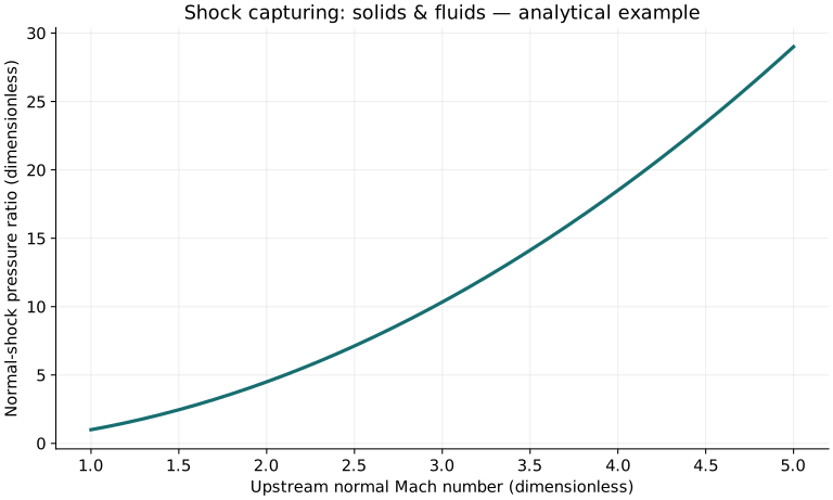
Twenty worked examples
Open a problem to see its defined inputs, assumptions, equation, numerical substitution, result, and interpretation. Values are illustrative analytical exercises.
Example 01. Burgers shock speed
Definitions & inputs. f(u)=u²/2,uL2,uR0 in consistent normalized units.
Choose the governing model and isolate the requested quantity.
Insert the stated inputs in consistent units or the explicitly defined normalized units.
Evaluate the expression; the result uses the units shown.
Interpretation. Compressive shock withuL>uR.
↑ Return to definitions and contentsExample 02. Shock position
Definitions & inputs. Initial x0=0,s1,t.4.
Choose the governing model and isolate the requested quantity.
Insert the stated inputs in consistent units or the explicitly defined normalized units.
Evaluate the expression; the result uses the units shown.
Interpretation. Constant-speed discontinuity.
↑ Return to definitions and contentsExample 03. Acoustic speed
Definitions & inputs. γ1.4,p100000Pa,ρ1.2kg/m³.
Choose the governing model and isolate the requested quantity.
Insert the stated inputs in consistent units or the explicitly defined normalized units.
Evaluate the expression; the result uses the units shown.
Interpretation. Ideal gas.
↑ Return to definitions and contentsExample 04. Maximum Euler speed
Definitions & inputs. u100m/s,c340m/s.
Choose the governing model and isolate the requested quantity.
Insert the stated inputs in consistent units or the explicitly defined normalized units.
Evaluate the expression; the result uses the units shown.
Interpretation. Bounds one-dimensional characteristics.
↑ Return to definitions and contentsExample 05. CFL time step
Definitions & inputs. Δx.01m,CFL.5,a500m/s.
Choose the governing model and isolate the requested quantity.
Insert the stated inputs in consistent units or the explicitly defined normalized units.
Evaluate the expression; the result uses the units shown.
Interpretation. Explicit method.
↑ Return to definitions and contentsExample 06. Courant number
Definitions & inputs. a2m/s,Δt.1s,Δx.5m.
Choose the governing model and isolate the requested quantity.
Insert the stated inputs in consistent units or the explicitly defined normalized units.
Evaluate the expression; the result uses the units shown.
Interpretation. Compare with method-specific limit.
↑ Return to definitions and contentsExample 07. Conservative update
Definitions & inputs. U1,dt/dx.1,right flux3,left flux2.
Choose the governing model and isolate the requested quantity.
Insert the stated inputs in consistent units or the explicitly defined normalized units.
Evaluate the expression; the result uses the units shown.
Interpretation. Normalized scalar example.
↑ Return to definitions and contentsExample 08. Upwind flux
Definitions & inputs. Positive advection a2,uL3.
Choose the governing model and isolate the requested quantity.
Insert the stated inputs in consistent units or the explicitly defined normalized units.
Evaluate the expression; the result uses the units shown.
Interpretation. Exact scalar upwind flux.
↑ Return to definitions and contentsExample 09. Rusanov scalar flux
Definitions & inputs. Advection a2,uL3,uR1.
Choose the governing model and isolate the requested quantity.
Insert the stated inputs in consistent units or the explicitly defined normalized units.
Evaluate the expression; the result uses the units shown.
Interpretation. Reduces to upwind with exact speed bound.
↑ Return to definitions and contentsExample 10. Minmod slope
Definitions & inputs. Candidate slopes2and−1.
Choose the governing model and isolate the requested quantity.
Insert the stated inputs in consistent units or the explicitly defined normalized units.
Evaluate the expression; the result uses the units shown.
Interpretation. Opposite signs flatten a local extremum.
↑ Return to definitions and contentsExample 11. Minmod same signs
Definitions & inputs. Candidate slopes2and1.
Choose the governing model and isolate the requested quantity.
Insert the stated inputs in consistent units or the explicitly defined normalized units.
Evaluate the expression; the result uses the units shown.
Interpretation. Choose smaller magnitude.
↑ Return to definitions and contentsExample 12. Pressure from energy
Definitions & inputs. γ1.4,ρE300000J/m³,ρ1,u100m/s.
Choose the governing model and isolate the requested quantity.
Insert the stated inputs in consistent units or the explicitly defined normalized units.
Evaluate the expression; the result uses the units shown.
Interpretation. Total energy includes kinetic energy.
↑ Return to definitions and contentsExample 13. Normal shock density ratio
Definitions & inputs. M1=2,γ1.4.
Choose the governing model and isolate the requested quantity.
Insert the stated inputs in consistent units or the explicitly defined normalized units.
Evaluate the expression; the result uses the units shown.
Interpretation. Ideal-gas stationary normal shock.
↑ Return to definitions and contentsExample 14. Normal shock pressure ratio
Definitions & inputs. Same upstream.
Choose the governing model and isolate the requested quantity.
Insert the stated inputs in consistent units or the explicitly defined normalized units.
Evaluate the expression; the result uses the units shown.
Interpretation. Irreversible pressure rise.
↑ Return to definitions and contentsExample 15. Bar wave speed
Definitions & inputs. E200GPa,ρ7800kg/m³.
Choose the governing model and isolate the requested quantity.
Insert the stated inputs in consistent units or the explicitly defined normalized units.
Evaluate the expression; the result uses the units shown.
Interpretation. Slender elastic bar.
↑ Return to definitions and contentsExample 16. Bar transit time
Definitions & inputs. L1m,c5000m/s.
Choose the governing model and isolate the requested quantity.
Insert the stated inputs in consistent units or the explicitly defined normalized units.
Evaluate the expression; the result uses the units shown.
Interpretation. One-way transit.
↑ Return to definitions and contentsExample 17. Impedance
Definitions & inputs. ρ7800kg/m³,c5000m/s.
Choose the governing model and isolate the requested quantity.
Insert the stated inputs in consistent units or the explicitly defined normalized units.
Evaluate the expression; the result uses the units shown.
Interpretation. Longitudinal mechanical impedance.
↑ Return to definitions and contentsExample 18. Stress reflection
Definitions & inputs. Z2=2Z1.
Choose the governing model and isolate the requested quantity.
Insert the stated inputs in consistent units or the explicitly defined normalized units.
Evaluate the expression; the result uses the units shown.
Interpretation. Positive reflected stress at higher impedance.
↑ Return to definitions and contentsExample 19. Matched interface
Definitions & inputs. Z2=Z1.
Choose the governing model and isolate the requested quantity.
Insert the stated inputs in consistent units or the explicitly defined normalized units.
Evaluate the expression; the result uses the units shown.
Interpretation. No reflection in this model.
↑ Return to definitions and contentsExample 20. Observed order
Definitions & inputs. Errors.04onh,.01onh/2.
Choose the governing model and isolate the requested quantity.
Insert the stated inputs in consistent units or the explicitly defined normalized units.
Evaluate the expression; the result uses the units shown.
Interpretation. Smooth-problem rate; shocks often reduce global convergence order.
↑ Return to definitions and contentsSymbols and units
Each derivation and problem defines its own symbols and inputs. Symbols may be reused with different meanings in other subjects. Keep units consistent, retain sufficient precision during calculation, and apply the stated validity limits.