PHYSICS / ENGINEERING / COMPUTING
Sensor types, measurement models and calibration
44 cumulative daily visits · View visitor map ↘
Explore a searchable atlas of sensing principles, measurement categories and applications, followed by derivations and twenty worked examples.
Matter pathway: atom → solid → liquid → gas → plasma. Quantum mechanics and quantum field theory provide foundations across the pathway; they are not additional phases. This is a connected modeling route, not a universal heating curve. Actual phases depend on pressure, composition, and kinetics.
Search the sensor atlas
90 sensor families across 10 measurement categories. Open an entry for its operating principle, governing equation, short derivation, assumptions, related physical subjects, practical applications, and references. Equations describe representative sensing modes; consult the cited source and device calibration for a specific instrument. Some entries are complete instruments rather than individual transducer elements.
Thermocouple
Thermal
Principle. Seebeck voltage measures a junction temperature difference; needs reference-junction compensation.
Practical applications. Furnaces and engine exhaust probes.
Governing equation & derivation
Symbols. S is Seebeck coefficient; temperatures refer to sensing and reference junctions.
Derivation. Integrate the difference of thermoelectric fields around the two-metal circuit; constant coefficient gives the linear approximation.
Assumptions & limits. Reference-junction compensation and material-specific calibration are required.
Related physical subjects. Heat transfer · Ray tracing · Material science · Plastic viscoelastic deformation · Rocket design · Hypersonic vehicle design · Internal combustion engine design · Optimization
Temperature and heat — reference / product families ↗ · Google this sensor ↗
↑ Sensor atlasResistance temperature detector (RTD)
Thermal
Principle. Metal resistance varies with temperature and is calibrated against a reference.
Practical applications. Platinum process thermometers and laboratory probes.
Governing equation & derivation
Symbols. R0 reference resistance; α local temperature coefficient.
Derivation. Linearize the calibrated resistance curve at T0 and invert its slope to estimate temperature.
Assumptions & limits. Limited temperature interval; lead resistance and self-heating bias the result.
Related physical subjects. Heat transfer · Ray tracing · Material science · Statistical physics · Statistics · Uncertainty quantification
Temperature and heat — reference / product families ↗ · Google this sensor ↗
↑ Sensor atlasThermistor
Thermal
Principle. A semiconductor resistor has a strong nonlinear temperature dependence.
Practical applications. Battery packs, appliances and medical thermometers.
Governing equation & derivation
Symbols. B beta coefficient in kelvin; T absolute temperature.
Derivation. Integrate dlnR/d(1/T)=B for an activated-resistance approximation.
Assumptions & limits. NTC beta law over a calibrated range; use a richer fit when needed.
Related physical subjects. Heat transfer · Ray tracing · Material science · Satellite design · Electric car motor design · Submarine design · Embedded software · Reliability
Temperature and heat — reference / product families ↗ · Google this sensor ↗
↑ Sensor atlasSemiconductor junction temperature sensor
Thermal
Principle. Junction voltage or paired-junction voltage difference provides a temperature signal.
Practical applications. Digital board thermometers and processor monitoring.
Governing equation & derivation
Symbols. r ratio of junction current densities; q elementary charge.
Derivation. Subtract two ideal diode voltage laws at different current densities to cancel the common saturation-current term.
Assumptions & limits. Matched junctions, appropriate ideality and calibrated parasitics.
Related physical subjects. Heat transfer · Ray tracing · Material science · Microelectronics · Computer chip design · Operating systems
Temperature and heat — reference / product families ↗ · Google this sensor ↗
↑ Sensor atlasThermopile infrared sensor
Thermal
Principle. Absorbed radiation heats thermocouple junctions relative to a reference.
Practical applications. Noncontact thermometers and infrared radiometers.
Governing equation & derivation
Symbols. N junction pairs, Rth thermal resistance, α absorptance, A area, Tt target and Ts sensor temperatures.
Derivation. Absorbed net radiant power creates a thermal rise; series thermocouples convert that rise to voltage.
Assumptions & limits. Ideal blackbody full-view target; real bandpass, view factor and emissivity need calibration.
Related physical subjects. Heat transfer · Ray tracing · Material science
Temperature and heat — reference / product families ↗ · Google this sensor ↗
↑ Sensor atlasBolometer / microbolometer
Thermal
Principle. Radiation-induced temperature rise changes an absorber’s resistance.
Practical applications. Uncooled thermal imaging cameras.
Governing equation & derivation
Symbols. Cth heat capacity, Gth conductance, αR resistance temperature coefficient.
Derivation. Balance absorber heat storage and loss, then linearize resistance with temperature.
Assumptions & limits. Small signal, fixed bath and negligible nonlinear electrothermal feedback.
Related physical subjects. Heat transfer · Ray tracing · Material science · Astrophysics · Quantum statistical physics
Temperature and heat — reference / product families ↗ · Google this sensor ↗
↑ Sensor atlasPyroelectric infrared sensor
Thermal
Principle. Changes in crystal polarization detect changes in absorbed radiant heating.
Practical applications. Passive-infrared motion detectors.
Governing equation & derivation
Symbols. p pyroelectric coefficient; A electrode area.
Derivation. Differentiate polarization charge Q=AP(T) with respect to time.
Assumptions & limits. Detects temperature changes; a steady target needs modulation and a thermal response model.
Related physical subjects. Heat transfer · Ray tracing · Material science
Temperature and heat — reference / product families ↗ · Google this sensor ↗
↑ Sensor atlasHeat-flux sensor
Thermal
Principle. A calibrated temperature gradient or thermopile voltage measures heat flow per area.
Practical applications. Building insulation and thermal test panels.
Governing equation & derivation
Symbols. k thermal conductivity and L sensing-layer thickness.
Derivation. Apply Fourier conduction through the calibrated layer; a thermopile measures its temperature drop.
Assumptions & limits. Approximately one-dimensional heat flow and known contact resistances.
Related physical subjects. Heat transfer · Ray tracing · Material science · Hypersonic vehicle design
Temperature and heat — reference / product families ↗ · Google this sensor ↗
↑ Sensor atlasStrain gauge
Mechanical
Principle. Deformation changes conductor resistance; a bridge resolves the small signal.
Practical applications. Structural monitoring and test coupons.
Governing equation & derivation
Symbols. GF gauge factor; ε axial strain.
Derivation. Differentiate resistance ρL/A and combine geometric and piezoresistive contributions into GF.
Assumptions & limits. Small strain, temperature compensation and appropriate bonding.
Related physical subjects. Solid mechanics · Continuum mechanics · Material science · Robotics · Rocket design · Ship design · Solid state physics · Survivability
TE Connectivity — mechanical sensor families — reference / product families ↗ · Google this sensor ↗
↑ Sensor atlasLoad cell
Mechanical
Principle. An elastic element converts force into measured strain or another calibrated displacement.
Practical applications. Weighing scales and test machines.
Governing equation & derivation
Symbols. E elastic modulus, A effective area, bridge excitation Vexc.
Derivation. An axial elastic member turns force into strain; a quarter bridge turns a small resistance change into voltage.
Assumptions & limits. Representative axial quarter-bridge model; commercial bending/full-bridge cells use different calibrated factors.
Related physical subjects. Solid mechanics · Continuum mechanics · Material science · Robotics · Plastic viscoelastic deformation · Statistics · Uncertainty quantification · Optimization
TE Connectivity — mechanical sensor families — reference / product families ↗ · Google this sensor ↗
↑ Sensor atlasPiezoresistive pressure sensor
Mechanical
Principle. Diaphragm stress changes semiconductor resistivity.
Practical applications. Automotive pressure modules and industrial transmitters.
Governing equation & derivation
Symbols. π coefficients relate longitudinal and transverse stress to resistance change.
Derivation. Pressure bends a diaphragm; its stress field enters the piezoresistive law and a bridge reads the imbalance.
Assumptions & limits. Requires diaphragm mechanics, crystal orientation and temperature calibration.
Related physical subjects. Solid mechanics · Continuum mechanics · Material science · Robotics · Shock capturing · Rocket design · Hypersonic vehicle design · Internal combustion engine design · Submarine design · Fluid mechanics · Gaseous state physics · Statistical physics
TE Connectivity — mechanical sensor families — reference / product families ↗ · Google this sensor ↗
↑ Sensor atlasCapacitive pressure sensor
Mechanical
Principle. Pressure deflects a diaphragm and changes electrode capacitance.
Practical applications. Low-pressure measurement and MEMS barometers.
Governing equation & derivation
Symbols. εd dielectric permittivity, w diaphragm displacement.
Derivation. Pressure moves a compliant electrode, changing electric-field spacing and stored charge per volt.
Assumptions & limits. Uniform-gap approximation; a real bent diaphragm requires area integration.
Related physical subjects. Solid mechanics · Continuum mechanics · Material science · Robotics
TE Connectivity — mechanical sensor families — reference / product families ↗ · Google this sensor ↗
↑ Sensor atlasPiezoelectric force sensor
Mechanical
Principle. Applied stress produces charge in a piezoelectric element; leakage limits static response.
Practical applications. Impact testing and machining-force measurement.
Governing equation & derivation
Symbols. dp charge coefficient, C total capacitance.
Derivation. Integrate piezoelectric polarization from applied force over the electrode.
Assumptions & limits. Dynamic or quasi-static measurement; leakage and charge-amplifier time constants limit DC response.
Related physical subjects. Solid mechanics · Continuum mechanics · Material science · Robotics · Shock capturing
TE Connectivity — mechanical sensor families — reference / product families ↗ · Google this sensor ↗
↑ Sensor atlasBourdon pressure element
Mechanical
Principle. Curvature of an elastic tube changes with internal pressure.
Practical applications. Mechanical pressure gauges with pointer or electrical readout.
Governing equation & derivation
Symbols. Sp calibrated tube-tip sensitivity; Gm linkage gain.
Derivation. Linearize elastic tube straightening around an operating point and apply the mechanical linkage ratio.
Assumptions & limits. Geometry-dependent local calibration, hysteresis and overload limits; not a universal tube law.
Related physical subjects. Solid mechanics · Continuum mechanics · Material science · Robotics
TE Connectivity — mechanical sensor families — reference / product families ↗ · Google this sensor ↗
↑ Sensor atlasLVDT displacement sensor
Mechanical
Principle. Core movement changes differential transformer coupling.
Practical applications. Valve position and dimensional metrology.
Governing equation & derivation
Symbols. M1,M2 mutual inductances; Ip excitation phasor.
Derivation. Subtract induced secondary voltages; near the null the coupling difference is proportional to core displacement.
Assumptions & limits. Demodulated linear range, stable excitation and limited magnetic saturation.
Related physical subjects. Solid mechanics · Continuum mechanics · Material science · Robotics · Plastic viscoelastic deformation
TE Connectivity — mechanical sensor families — reference / product families ↗ · Google this sensor ↗
↑ Sensor atlasPotentiometric position sensor
Mechanical
Principle. A moving contact samples a resistive voltage divider.
Practical applications. Control knobs and linear position transducers.
Governing equation & derivation
Symbols. x wiper position along uniform track length L.
Derivation. Use the resistive voltage-divider ratio Rsegment/Rtotal=x/L.
Assumptions & limits. Negligible loading, uniform track and good wiper contact.
Related physical subjects. Solid mechanics · Continuum mechanics · Material science · Robotics
TE Connectivity — mechanical sensor families — reference / product families ↗ · Google this sensor ↗
↑ Sensor atlasCapacitive displacement sensor
Mechanical
Principle. Electrode gap or overlap changes capacitance.
Practical applications. Precision positioning and thickness measurement.
Governing equation & derivation
Symbols. d gap; A overlap area.
Derivation. Integrate a uniform plate field to obtain charge, then divide by voltage and invert.
Assumptions & limits. Parallel plates, small fringe contribution and known dielectric.
Related physical subjects. Solid mechanics · Continuum mechanics · Material science · Robotics
TE Connectivity — mechanical sensor families — reference / product families ↗ · Google this sensor ↗
↑ Sensor atlasInductive proximity sensor
Mechanical
Principle. Conductive or magnetic targets alter an excited electromagnetic field.
Practical applications. Industrial part detection.
Governing equation & derivation
Symbols. N turns, magnetic reluctance Rm, oscillator capacitance C.
Derivation. A target changes the coil’s magnetic or loss environment, shifting inductance or oscillator damping.
Assumptions & limits. Representative resonance model; conductive targets also produce eddy-current losses and require calibration.
Related physical subjects. Solid mechanics · Continuum mechanics · Material science · Robotics
TE Connectivity — mechanical sensor families — reference / product families ↗ · Google this sensor ↗
↑ Sensor atlasEddy-current displacement sensor
Mechanical
Principle. A conductive target’s induced currents alter probe impedance.
Practical applications. Shaft clearance and vibration monitoring.
Governing equation & derivation
Symbols. δ skin depth, σe electrical conductivity, d target gap.
Derivation. Maxwell induction creates target currents whose secondary field changes complex probe impedance.
Assumptions & limits. Gap inference requires a calibrated geometry-dependent impedance function; skin depth alone is not a displacement calibration.
Related physical subjects. Solid mechanics · Continuum mechanics · Material science · Robotics
TE Connectivity — mechanical sensor families — reference / product families ↗ · Google this sensor ↗
↑ Sensor atlasOptical encoder
Mechanical
Principle. A patterned scale modulates light to encode angular or linear position.
Practical applications. Servo motors and machine tools.
Governing equation & derivation
Symbols. n counted increments, N resolved increments per revolution.
Derivation. A periodic optical pattern converts each resolved transition into a known angle increment.
Assumptions & limits. Specify quadrature decoding, index reference, direction and missed-count limits.
Related physical subjects. Solid mechanics · Continuum mechanics · Material science · Robotics · Control theory · Embedded software
TE Connectivity — mechanical sensor families — reference / product families ↗ · Google this sensor ↗
↑ Sensor atlasMagnetic encoder
Mechanical
Principle. A magnetic pattern and field-sensitive elements encode position.
Practical applications. Motor-angle feedback in dusty environments.
Governing equation & derivation
Symbols. Vsin,Vcos offset-corrected quadrature magnetic signals.
Derivation. Resolve two orthogonal field components and recover phase from their ratio with quadrant information.
Assumptions & limits. One-pole-pair model; multipole patterns, offsets and harmonics need correction.
Related physical subjects. Solid mechanics · Continuum mechanics · Material science · Robotics · Car design · Electric car motor design
TE Connectivity — mechanical sensor families — reference / product families ↗ · Google this sensor ↗
↑ Sensor atlasFiber Bragg grating sensor
Mechanical
Principle. Strain or temperature shifts the wavelength reflected by a grating in optical fiber.
Practical applications. Distributed structural monitoring; cross-sensitivity needs compensation.
Governing equation & derivation
Symbols. Λ grating period, pe photoelastic factor, α expansion and ξ thermo-optic coefficient.
Derivation. Constructive Bragg reflection fixes wavelength; differentiate index and period changes.
Assumptions & limits. Small strain/temperature changes; temperature–strain cross-sensitivity needs separation.
Related physical subjects. Solid mechanics · Continuum mechanics · Material science · Robotics
TE Connectivity — mechanical sensor families — reference / product families ↗ · Google this sensor ↗
↑ Sensor atlasTactile array
Mechanical
Principle. An array maps local force or contact through resistive, capacitive or optical elements.
Practical applications. Robot grippers and touch surfaces.
Governing equation & derivation
Symbols. pi calibrated local pressure, Ai pixel area.
Derivation. Convert each cell’s signal to pressure and integrate over contact area.
Assumptions & limits. Cell transfer laws depend on resistive, capacitive or optical construction; saturation and cross-talk matter.
Related physical subjects. Solid mechanics · Continuum mechanics · Material science · Robotics
TE Connectivity — mechanical sensor families — reference / product families ↗ · Google this sensor ↗
↑ Sensor atlasCapacitive MEMS accelerometer
Inertial
Principle. A proof mass deflects under specific force and changes differential capacitance.
Practical applications. Phones, vibration loggers and inertial modules.
Governing equation & derivation
Symbols. m proof mass,b damping,k stiffness.
Derivation. Newton’s law in the accelerating sensor frame gives a driven oscillator; gap capacitances read x.
Assumptions & limits. Low-frequency approximation below resonance; measures specific force with gravity handled by navigation conventions.
Related physical subjects. Robotics · Control theory · Satellite design · Car design · Continuum mechanics · Embedded software
Motion and navigation — reference / product families ↗ · Google this sensor ↗
↑ Sensor atlasPiezoelectric accelerometer
Inertial
Principle. Proof-mass force produces piezoelectric charge for dynamic acceleration.
Practical applications. Machinery vibration testing.
Governing equation & derivation
Symbols. m effective proof mass and dp piezoelectric coefficient.
Derivation. Inertial force ma loads the piezoelectric element, producing proportional charge.
Assumptions & limits. Dynamic band only, below structural resonance and above leakage cutoff.
Related physical subjects. Robotics · Control theory · Satellite design · Car design · Satellite spallation · Reliability
Motion and navigation — reference / product families ↗ · Google this sensor ↗
↑ Sensor atlasMEMS vibrating gyroscope
Inertial
Principle. Coriolis coupling between driven and sensed modes measures angular rate.
Practical applications. Drones and inertial navigation modules.
Governing equation & derivation
Symbols. Ω rotation rate, vd driven proof-mass velocity perpendicular to the rate axis.
Derivation. Coriolis acceleration couples the driven mode into the sense mode.
Assumptions & limits. Small angular rates and calibrated resonant transfer function; quadrature and bias need correction.
Related physical subjects. Robotics · Control theory · Satellite design · Car design
Motion and navigation — reference / product families ↗ · Google this sensor ↗
↑ Sensor atlasFiber-optic gyroscope
Inertial
Principle. Counter-propagating light acquires a rotation-dependent Sagnac phase difference.
Practical applications. Navigation-grade inertial systems.
Governing equation & derivation
Symbols. Aeff oriented loop area summed over turns; λ vacuum wavelength.
Derivation. Counterpropagating paths acquire a Sagnac time difference and hence an optical phase difference.
Assumptions & limits. Reciprocal-path approximation; polarization and thermal nonreciprocity require control.
Related physical subjects. Robotics · Control theory · Satellite design · Car design
Motion and navigation — reference / product families ↗ · Google this sensor ↗
↑ Sensor atlasRing-laser gyroscope
Inertial
Principle. Rotation shifts the frequencies of counter-propagating cavity modes.
Practical applications. Aircraft inertial reference systems.
Governing equation & derivation
Symbols. A ring area, P perimeter, λ wavelength.
Derivation. Sagnac path-time asymmetry splits counterpropagating cavity resonances.
Assumptions & limits. Ideal ring; lock-in and bias require engineering compensation.
Related physical subjects. Robotics · Control theory · Satellite design · Car design
Motion and navigation — reference / product families ↗ · Google this sensor ↗
↑ Sensor atlasInclinometer
Inertial
Principle. Gravity-sensitive acceleration or a fluid/mechanical reference estimates tilt under suitable dynamics.
Practical applications. Platform leveling and geotechnical monitoring.
Governing equation & derivation
Symbols. ax,az calibrated gravity-vector components in a chosen sign convention.
Derivation. Project static gravity onto two axes and recover orientation.
Assumptions & limits. Translational acceleration invalidates a gravity-only tilt estimate.
Related physical subjects. Robotics · Control theory · Satellite design · Car design · Ship design · Submarine design
Motion and navigation — reference / product families ↗ · Google this sensor ↗
↑ Sensor atlasGNSS receiver
Inertial
Principle. Correlates satellite signals and solves pseudoranges for position and clock offset.
Practical applications. Survey receivers and navigation devices.
Governing equation & derivation
Symbols. ρi pseudorange, ri satellite position, δt receiver clock offset.
Derivation. Convert measured code delay to length and solve simultaneous position/clock equations.
Assumptions & limits. Satellite clock, relativity, atmosphere, ephemeris and multipath corrections are required.
Related physical subjects. Robotics · Control theory · Satellite design · Car design · Astrodynamics · Trajectory calculation · Ship design · General relativity
Motion and navigation — reference / product families ↗ · Google this sensor ↗
↑ Sensor atlasStar tracker
Inertial
Principle. Star-image patterns and catalog matching estimate spacecraft attitude.
Practical applications. Satellite attitude determination.
Governing equation & derivation
Symbols. si catalog star direction, bi measured body-frame direction, R attitude rotation.
Derivation. Project star images to unit vectors and fit a common rotation by weighted least squares.
Assumptions & limits. Identified stars, calibrated optics, R orthogonal with determinant one and appropriate noise weights.
Related physical subjects. Robotics · Control theory · Satellite design · Car design · Astrodynamics · Trajectory calculation
Motion and navigation — reference / product families ↗ · Google this sensor ↗
↑ Sensor atlasPhotodiode
Optical
Principle. Absorbed photons create collected electron-hole pairs.
Practical applications. Optical power meters and fiber receivers.
Governing equation & derivation
Symbols. ηq quantum efficiency; R responsivity.
Derivation. Divide optical power by photon energy and multiply detected photon rate by electron charge.
Assumptions & limits. Linear spectral response; dark current, saturation and bandwidth remain separate.
Related physical subjects. Optics · Ray tracing · Atomic physics · Quantum mechanics · Plasma physics · Communication systems · Quantum statistical physics
Optical detector families — reference / product families ↗ · Google this sensor ↗
↑ Sensor atlasAvalanche photodiode
Optical
Principle. Internal impact ionization multiplies photocarrier current below breakdown operation.
Practical applications. Optical receivers and ranging instruments.
Governing equation & derivation
Symbols. M avalanche gain.
Derivation. Multiply primary photocarrier current by mean impact-ionization gain.
Assumptions & limits. Below breakdown linear mode; gain noise, temperature and bias stability matter.
Related physical subjects. Optics · Ray tracing · Atomic physics · Quantum mechanics
Optical detector families — reference / product families ↗ · Google this sensor ↗
↑ Sensor atlasSingle-photon avalanche diode (SPAD)
Optical
Principle. A photon can trigger a quenched Geiger-mode avalanche.
Practical applications. Time-of-flight modules and photon counting.
Governing equation & derivation
Symbols. PDE detection efficiency, τd nonparalyzable dead time.
Derivation. Detected arrivals occupy the detector for a dead interval, reducing count throughput.
Assumptions & limits. Simplified stationary model; afterpulsing, pile-up and timing response need characterization.
Related physical subjects. Optics · Ray tracing · Atomic physics · Quantum mechanics · Quantum computing
Optical detector families — reference / product families ↗ · Google this sensor ↗
↑ Sensor atlasSilicon photomultiplier
Optical
Principle. Many quenched avalanche microcells sum signals from detected photons.
Practical applications. Scintillation readout and low-light instruments.
Governing equation & derivation
Symbols. Ncell microcells; Nγ short-pulse incident photons.
Derivation. Treat independent photon assignment to cells as Poisson occupancy; a cell fires if at least one photon triggers it.
Assumptions & limits. No recharge during pulse, cross-talk or afterpulsing in this approximation.
Related physical subjects. Optics · Ray tracing · Atomic physics · Quantum mechanics
Optical detector families — reference / product families ↗ · Google this sensor ↗
↑ Sensor atlasPhotomultiplier tube
Optical
Principle. Photoelectrons are multiplied through a vacuum dynode chain or related gain structure.
Practical applications. Spectroscopy and particle detectors.
Governing equation & derivation
Symbols. δ mean gain per dynode,n stages.
Derivation. A photocathode converts photons to electrons and repeated secondary emission multiplies their number.
Assumptions & limits. Stage-independent mean gain model; dark counts, excess noise and saturation omitted.
Related physical subjects. Optics · Ray tracing · Atomic physics · Quantum mechanics · Quantum computing
Optical detector families — reference / product families ↗ · Google this sensor ↗
↑ Sensor atlasCCD image sensor
Optical
Principle. Photocharge is transferred between potential wells to a readout.
Practical applications. Scientific cameras and spectroscopy.
Governing equation & derivation
Symbols. Ne collected electrons,t exposure.
Derivation. Integrate detected photon rate; Poisson arrivals give shot-noise standard deviation.
Assumptions & limits. Add dark/read noise and charge-transfer losses; avoid full-well saturation.
Related physical subjects. Optics · Ray tracing · Atomic physics · Quantum mechanics · Astrophysics · General relativity
Optical detector families — reference / product families ↗ · Google this sensor ↗
↑ Sensor atlasCMOS image sensor
Optical
Principle. Pixel photodetectors and local transistor readout form an image.
Practical applications. Phone cameras and machine vision.
Governing equation & derivation
Symbols. Cnode conversion-node capacitance.
Derivation. Photons generate charge that is converted into a pixel voltage and read electronically.
Assumptions & limits. Representative conversion gain; read noise, rolling/global shutter and pixel circuitry differ.
Related physical subjects. Optics · Ray tracing · Atomic physics · Quantum mechanics
Optical detector families — reference / product families ↗ · Google this sensor ↗
↑ Sensor atlasPosition-sensitive photodetector
Optical
Principle. Photocurrent division or segmented detection estimates a light spot’s location.
Practical applications. Alignment instruments and optical tracking.
Governing equation & derivation
Symbols. L active length; IR,IL electrode photocurrents.
Derivation. Normalize current imbalance by total intensity to infer spot position.
Assumptions & limits. Calibrated linear lateral-effect model, spot wholly inside active area.
Related physical subjects. Optics · Ray tracing · Atomic physics · Quantum mechanics
Optical detector families — reference / product families ↗ · Google this sensor ↗
↑ Sensor atlasSpectrometer sensor
Optical
Principle. Wavelength-dependent optics or filters separate a spectrum for detection.
Practical applications. Chemical identification and optical characterization.
Governing equation & derivation
Symbols. d grating period,m diffraction order,α incidence,β diffraction angle in the chosen convention.
Derivation. Adjacent grooves produce a path difference; integer wavelengths interfere constructively.
Assumptions & limits. Representative grating spectrometer; resolution also depends on slit, aberrations, pixel sampling and illuminated grooves.
Related physical subjects. Optics · Ray tracing · Atomic physics · Quantum mechanics · Material science · Gaseous state physics · Solid state physics · Plasma physics · Astrophysics · Chemical kinetics · Quantum statistical physics
Optical detector families — reference / product families ↗ · Google this sensor ↗
↑ Sensor atlasLidar / optical time-of-flight
Optical
Principle. Travel time or modulation phase of returned light gives range.
Practical applications. Mapping instruments and robot navigation.
Governing equation & derivation
Symbols. Δt round-trip delay,n medium refractive index.
Derivation. Light travels to the target and back at speed c/n; divide total path length by two.
Assumptions & limits. Timing offsets, multiple returns, ambient light and target reflectance matter.
Related physical subjects. Optics · Ray tracing · Atomic physics · Quantum mechanics · Robotics
Optical detector families — reference / product families ↗ · Google this sensor ↗
↑ Sensor atlasInterferometric displacement sensor
Optical
Principle. Optical path differences modulate fringe phase.
Practical applications. Nanometre positioning and precision metrology.
Governing equation & derivation
Symbols. Δx mirror displacement in a double-pass path.
Derivation. Motion changes round-trip optical path by2nΔx; multiply by2π/λ.
Assumptions & limits. Phase unwrapping and environmental refractive-index correction required.
Related physical subjects. Optics · Ray tracing · Atomic physics · Quantum mechanics · Shock capturing · Satellite spallation · General relativity
Optical detector families — reference / product families ↗ · Google this sensor ↗
↑ Sensor atlasPolarization sensor
Optical
Principle. Multiple analyzer states infer polarization components.
Practical applications. Stress imaging and surface inspection.
Governing equation & derivation
Symbols. S0,S1,S2 Stokes parameters,θ linear analyzer angle.
Derivation. Resolve the polarization coherence matrix onto the analyzer direction.
Assumptions & limits. Linear analyzers alone cannot measure circular StokesS3; add a retarder for full polarimetry.
Related physical subjects. Optics · Ray tracing · Atomic physics · Quantum mechanics
Optical detector families — reference / product families ↗ · Google this sensor ↗
↑ Sensor atlasCondenser microphone
Acoustic
Principle. Sound pressure changes diaphragm capacitance.
Practical applications. Measurement microphones and audio recording.
Governing equation & derivation
Symbols. x diaphragm deflection.
Derivation. Acoustic pressure drives diaphragm mechanics and changes electrode spacing.
Assumptions & limits. Small motion; bias circuit and mechanical frequency response set pressure sensitivity.
Related physical subjects. Fluid mechanics · Solid mechanics · Ship design · Submarine design
Acoustic transducers — reference / product families ↗ · Google this sensor ↗
↑ Sensor atlasDynamic microphone
Acoustic
Principle. Moving-coil induction converts diaphragm velocity into voltage.
Practical applications. Audio microphones and acoustic systems.
Governing equation & derivation
Symbols. B gap flux density,ℓ active wire length,v coil velocity.
Derivation. Motion through magnetic flux induces an EMF proportional to velocity.
Assumptions & limits. Lumped moving-coil model; diaphragm/acoustic loading relates pressure to velocity.
Related physical subjects. Fluid mechanics · Solid mechanics · Ship design · Submarine design
Acoustic transducers — reference / product families ↗ · Google this sensor ↗
↑ Sensor atlasPiezoelectric acoustic sensor
Acoustic
Principle. Acoustic pressure or strain produces charge.
Practical applications. Contact pickups and ultrasonic transducers.
Governing equation & derivation
Symbols. p applied pressure,A loaded area.
Derivation. Pressure creates forceAp; piezoelectric charge is dp times force.
Assumptions & limits. Dynamic frequency response and boundary constraints affect sensitivity.
Related physical subjects. Fluid mechanics · Solid mechanics · Ship design · Submarine design
Acoustic transducers — reference / product families ↗ · Google this sensor ↗
↑ Sensor atlasHydrophone
Acoustic
Principle. An underwater transducer converts acoustic pressure into an electrical signal.
Practical applications. Ocean acoustics and tank measurements.
Governing equation & derivation
Symbols. M complex calibrated sensitivity in V/Pa.
Derivation. Solve acoustic–mechanical–electrical transduction, then express the resulting frequency-dependent transfer function.
Assumptions & limits. Sensitivity is a calibration function, not a universal constant; pressure, temperature and direction matter.
Related physical subjects. Fluid mechanics · Solid mechanics · Ship design · Submarine design
Acoustic transducers — reference / product families ↗ · Google this sensor ↗
↑ Sensor atlasUltrasonic distance sensor
Acoustic
Principle. Echo delay measures round-trip propagation time in a known medium.
Practical applications. Parking aids and level gauges.
Governing equation & derivation
Symbols. cs sound speed,Δt echo delay.
Derivation. Divide round-trip acoustic propagation length by two.
Assumptions & limits. Sound speed depends on medium and temperature; blanking and multiple echoes matter.
Related physical subjects. Fluid mechanics · Solid mechanics · Ship design · Submarine design
Acoustic transducers — reference / product families ↗ · Google this sensor ↗
↑ Sensor atlasAcoustic-emission sensor
Acoustic
Principle. Detects transient elastic waves released by localized material events.
Practical applications. Crack monitoring and pressure-vessel testing.
Governing equation & derivation
Symbols. r event position,ri sensor positions.
Derivation. Compare travel times of an elastic disturbance to estimate source location.
Assumptions & limits. Known wave mode and speed; anisotropy, dispersion and threshold timing complicate localization.
Related physical subjects. Fluid mechanics · Solid mechanics · Ship design · Submarine design · Material science · Satellite spallation · Reliability · Survivability
Acoustic transducers — reference / product families ↗ · Google this sensor ↗
↑ Sensor atlasHall-effect sensor
Electrical
Principle. Magnetic field deflects charge carriers and creates a transverse voltage.
Practical applications. Contactless current sensors and position switches.
Governing equation & derivation
Symbols. I bias current,B perpendicular field,n carrier density,t plate thickness.
Derivation. Balance transverse Lorentz force with the Hall electric field and integrate across the plate.
Assumptions & limits. Single-carrier idealization; sign, geometry factor, offset and temperature require calibration.
Related physical subjects. Electrical engineering · Microelectronics · Electric car motor design · Solid state physics
Electrical and magnetic sensing — reference / product families ↗ · Google this sensor ↗
↑ Sensor atlasAnisotropic magnetoresistive sensor
Electrical
Principle. Resistance changes with magnetization orientation relative to current.
Practical applications. Compasses and angle sensing.
Governing equation & derivation
Symbols. θ between magnetization and current.
Derivation. Spin-dependent scattering produces an orientation-dependent longitudinal resistance.
Assumptions & limits. Magnetization must follow the assumed field state; hysteresis and bridge geometry matter.
Related physical subjects. Electrical engineering · Microelectronics · Electric car motor design
Electrical and magnetic sensing — reference / product families ↗ · Google this sensor ↗
↑ Sensor atlasGiant / tunnel magnetoresistive sensor
Electrical
Principle. Spin-dependent transport changes resistance with magnetic alignment.
Practical applications. Magnetic read heads and angle sensors.
Governing equation & derivation
Symbols. P/AP parallel/antiparallel limits.
Derivation. A simple angular interpolation represents spin-dependent relative layer alignment.
Assumptions & limits. Phenomenological resistance law; actual tunneling conductance and bias dependence may differ.
Related physical subjects. Electrical engineering · Microelectronics · Electric car motor design
Electrical and magnetic sensing — reference / product families ↗ · Google this sensor ↗
↑ Sensor atlasFluxgate magnetometer
Electrical
Principle. A driven magnetic core’s saturation response reveals a small external field.
Practical applications. Geophysical and spacecraft field measurement.
Governing equation & derivation
Symbols. V2ω demodulated second-harmonic voltage,KB calibrated sensitivity.
Derivation. Symmetric core saturation has balanced half-cycles; a small external field breaks symmetry and generates an even harmonic.
Assumptions & limits. Small-field calibrated operating range, drive stability and core hysteresis constraints.
Related physical subjects. Electrical engineering · Microelectronics · Electric car motor design
Electrical and magnetic sensing — reference / product families ↗ · Google this sensor ↗
↑ Sensor atlasSQUID magnetometer
Electrical
Principle. Superconducting quantum interference converts tiny flux changes into an electrical response.
Practical applications. Magnetoencephalography and low-field research.
Governing equation & derivation
Symbols. I0 junction critical current,Φ loop flux.
Derivation. Add two Josephson supercurrents subject to flux-dependent phase difference.
Assumptions & limits. Symmetric low-inductance DC-SQUID idealization; flux-locked loops linearize a periodic response.
Related physical subjects. Electrical engineering · Microelectronics · Electric car motor design · Quantum computing
Electrical and magnetic sensing — reference / product families ↗ · Google this sensor ↗
↑ Sensor atlasCurrent shunt
Electrical
Principle. A calibrated low resistance converts current to a measured voltage drop.
Practical applications. Battery monitoring and power converters.
Governing equation & derivation
Symbols. R calibrated shunt resistance.
Derivation. Ohm’s law converts current to differential voltage; Joule heating changes temperature.
Assumptions & limits. Four-wire sensing, bandwidth, thermoelectric offsets and resistance drift matter.
Related physical subjects. Electrical engineering · Microelectronics · Electric car motor design · Control theory · Computer chip design · Operating systems · Antenna design · Uncertainty quantification · Optimization
Electrical and magnetic sensing — reference / product families ↗ · Google this sensor ↗
↑ Sensor atlasCurrent transformer
Electrical
Principle. Alternating primary current induces a scaled secondary current.
Practical applications. AC power metering; cannot measure steady DC by ordinary transformer action.
Governing equation & derivation
Symbols. Np,Ns turns; winding current signs follow flux convention.
Derivation. Ampere-turn balance under high core permeability gives the secondary current ratio.
Assumptions & limits. AC only for ordinary transformers; burden, saturation and magnetizing current create errors.
Related physical subjects. Electrical engineering · Microelectronics · Electric car motor design
Electrical and magnetic sensing — reference / product families ↗ · Google this sensor ↗
↑ Sensor atlasRogowski coil
Electrical
Principle. An air-core winding measures dI/dt and uses integration to recover AC/pulse current.
Practical applications. High-current transient measurement.
Governing equation & derivation
Symbols. M mutual inductance.
Derivation. Faraday induction measures changing current; an integrator reconstructs current up to an initial constant.
Assumptions & limits. Cannot recover DC from induction alone; integrator drift and bandwidth matter.
Related physical subjects. Electrical engineering · Microelectronics · Electric car motor design · Plasma physics
Electrical and magnetic sensing — reference / product families ↗ · Google this sensor ↗
↑ Sensor atlasElectric-field probe
Electrical
Principle. Capacitive or electro-optic coupling samples an electric field.
Practical applications. EMC testing and field mapping.
Governing equation & derivation
Symbols. E normal electric field,A effective electrode area.
Derivation. Induced electrode charge follows electric displacement flux; read charge or its time derivative.
Assumptions & limits. Representative capacitive probe; field disturbance and geometry factor need calibration.
Related physical subjects. Electrical engineering · Microelectronics · Electric car motor design · Antenna design · Communication systems
Electrical and magnetic sensing — reference / product families ↗ · Google this sensor ↗
↑ Sensor atlasRadar sensor
Electrical
Principle. Radio echo delay, phase and Doppler reveal range and radial speed.
Practical applications. Automotive ranging and industrial level measurement.
Governing equation & derivation
Symbols. vr radial closing speed,λ wavelength.
Derivation. Round-trip delay gives range and two-way phase rate gives monostatic Doppler.
Assumptions & limits. Signs depend on convention; FMCW range needs chirp-slope processing and Doppler separation.
Related physical subjects. Electrical engineering · Microelectronics · Electric car motor design · Astrodynamics · Trajectory calculation · Car design · Communication systems
Electrical and magnetic sensing — reference / product families ↗ · Google this sensor ↗
↑ Sensor atlasCapacitive humidity sensor
Environmental
Principle. Sorbed water changes a dielectric’s permittivity.
Practical applications. HVAC and weather stations.
Governing equation & derivation
Symbols. RH relative humidity; εr calibrated sorption-dependent permittivity.
Derivation. Water uptake changes dielectric polarization and capacitance.
Assumptions & limits. Material-specific temperature, hysteresis and contamination dependence; not a universal linearRHlaw.
Related physical subjects. Fluid mechanics · Gaseous state physics · Chemical kinetics
Environmental, gas and flow sensors — reference / product families ↗ · Google this sensor ↗
↑ Sensor atlasChilled-mirror dew-point sensor
Environmental
Principle. Optical detection controls a mirror at the onset of condensation.
Practical applications. Reference humidity metrology.
Governing equation & derivation
Symbols. Td dew point,Ta ambient temperature,psat saturation pressure.
Derivation. Condensation identifies vapor partial pressure as saturation pressure atTd; normalize to ambient saturation.
Assumptions & limits. Distinguish dew from frost and include pressure/composition corrections where relevant.
Related physical subjects. Fluid mechanics · Gaseous state physics · Chemical kinetics
Environmental, gas and flow sensors — reference / product families ↗ · Google this sensor ↗
↑ Sensor atlasThermal mass-flow sensor
Environmental
Principle. Flow modifies heat transport around a heated element.
Practical applications. Gas metering and liquid dosing modules.
Governing equation & derivation
Symbols. mdot mass flow,cp heat capacity.
Derivation. A calorimetric energy balance relates added heat to transported enthalpy plus losses.
Assumptions & limits. Representative calorimetric mode; bypass geometry, fluid properties and heat losses require calibration.
Related physical subjects. Fluid mechanics · Gaseous state physics · Chemical kinetics
Environmental, gas and flow sensors — reference / product families ↗ · Google this sensor ↗
↑ Sensor atlasDifferential-pressure flowmeter
Environmental
Principle. A calibrated restriction maps pressure drop to flow.
Practical applications. Process pipes and ventilation ducts.
Governing equation & derivation
Symbols. Ao orifice area,β diameter ratio,Cd discharge coefficient.
Derivation. Combine continuity and Bernoulli across a restriction, then correct contraction/losses empirically.
Assumptions & limits. Incompressible calibrated orifice regime; compressible flows need expansion correction.
Related physical subjects. Fluid mechanics · Gaseous state physics · Chemical kinetics
Environmental, gas and flow sensors — reference / product families ↗ · Google this sensor ↗
↑ Sensor atlasElectromagnetic flowmeter
Environmental
Principle. Conducting liquid moving through a magnetic field induces a voltage.
Practical applications. Water and process-fluid metering.
Governing equation & derivation
Symbols. B transverse field,D electrode spacing.
Derivation. Conducting fluid motion induces a transverse motional EMF.
Assumptions & limits. Full conductive pipe, suitable electrode contact and calibrated velocity profile.
Related physical subjects. Fluid mechanics · Gaseous state physics · Chemical kinetics
Environmental, gas and flow sensors — reference / product families ↗ · Google this sensor ↗
↑ Sensor atlasCoriolis mass-flowmeter
Environmental
Principle. Flow-driven motion in a vibrating tube reveals mass flow.
Practical applications. Chemical-process and custody-transfer instruments.
Governing equation & derivation
Symbols. Δφ measured tube-motion phase imbalance,Km calibrated sensitivity.
Derivation. Flow through a driven vibrating tube produces Coriolis coupling proportional to mass throughput in the linear regime.
Assumptions & limits. Tube geometry, stiffness, density and damping setKm; no universal phase constant.
Related physical subjects. Fluid mechanics · Gaseous state physics · Chemical kinetics · Internal combustion engine design
Environmental, gas and flow sensors — reference / product families ↗ · Google this sensor ↗
↑ Sensor atlasUltrasonic flowmeter
Environmental
Principle. Transit-time difference or Doppler shift measures fluid motion.
Practical applications. Clamp-on pipe meters.
Governing equation & derivation
Symbols. L acoustic path; tplus downstream,tminus upstream.
Derivation. Subtract reciprocal transit times to cancel sound speed in a uniform-flow model.
Assumptions & limits. Known path angle; cross-sectional mean flow needs a profile correction.
Related physical subjects. Fluid mechanics · Gaseous state physics · Chemical kinetics · Ship design · Liquid state physics
Environmental, gas and flow sensors — reference / product families ↗ · Google this sensor ↗
↑ Sensor atlasOptical particulate sensor
Environmental
Principle. Scattered light from particles estimates size/count or mass under a calibration model.
Practical applications. Air-quality monitors.
Governing equation & derivation
Symbols. N illuminated particle count; differential scattering cross section depends on size and refractive index.
Derivation. Sum single-particle scattered power into the detector’s collection angle.
Assumptions & limits. Dilute single scattering; inferred mass needs particle size, density and optical calibration.
Related physical subjects. Fluid mechanics · Gaseous state physics · Chemical kinetics
Environmental, gas and flow sensors — reference / product families ↗ · Google this sensor ↗
↑ Sensor atlasNondispersive infrared gas sensor
Environmental
Principle. Gas-specific absorption in selected infrared bands estimates concentration.
Practical applications. CO₂ monitors and process gas instruments.
Governing equation & derivation
Symbols. κ absorption coefficient per concentration,cg concentration,L path.
Derivation. Integrate Beer–Lambert attenuation and invert the logarithm.
Assumptions & limits. Band-integrated response, temperature, pressure and overlapping gases need compensation.
Related physical subjects. Fluid mechanics · Gaseous state physics · Chemical kinetics
Environmental, gas and flow sensors — reference / product families ↗ · Google this sensor ↗
↑ Sensor atlasPhotoacoustic gas sensor
Environmental
Principle. Modulated absorption creates pressure waves measured acoustically.
Practical applications. Compact gas analyzers.
Governing equation & derivation
Symbols. αabs absorption coefficient,Pmod modulated optical power,K cell response.
Derivation. Absorbed periodic heat drives gas expansion and an acoustic response read by a microphone.
Assumptions & limits. Small absorption and a calibrated acoustic/thermal transfer function.
Related physical subjects. Fluid mechanics · Gaseous state physics · Chemical kinetics
Environmental, gas and flow sensors — reference / product families ↗ · Google this sensor ↗
↑ Sensor atlasMetal-oxide gas sensor
Environmental
Principle. Surface reactions change a heated semiconductor’s conductance.
Practical applications. VOC indicators; selectivity and humidity cross-sensitivity require care.
Governing equation & derivation
Symbols. A,b empirical fit parameters,cg target concentration in stated units.
Derivation. Surface reaction and carrier depletion yield a calibrated log–log response over a limited range.
Assumptions & limits. Not universal kinetics; humidity, temperature, mixed gases and aging affect selectivity.
Related physical subjects. Fluid mechanics · Gaseous state physics · Chemical kinetics
Environmental, gas and flow sensors — reference / product families ↗ · Google this sensor ↗
↑ Sensor atlasElectrochemical gas sensor
Environmental
Principle. A target gas participates in an electrochemical reaction producing current or potential.
Practical applications. Portable gas detectors.
Governing equation & derivation
Symbols. ne electrons per reaction,F Faraday constant,Dg diffusivity.
Derivation. Diffusion-limited transport through a layer gives fluxDgcg/L; Faraday’s law converts molar flux to current.
Assumptions & limits. Representative steady diffusion-limited sensor; membrane partition and electrode kinetics can dominate.
Related physical subjects. Fluid mechanics · Gaseous state physics · Chemical kinetics
Environmental, gas and flow sensors — reference / product families ↗ · Google this sensor ↗
↑ Sensor atlasSoil-moisture dielectric sensor
Environmental
Principle. Dielectric response estimates volumetric water content after soil-specific calibration.
Practical applications. Irrigation monitoring.
Governing equation & derivation
Symbols. θv volumetric water fraction,εeff effective permittivity,EC conductivity.
Derivation. Water’s dielectric response changes capacitance or propagation; invert a soil-specific mixing/calibration relation.
Assumptions & limits. Texture, salinity, density and bound water prevent one universal conversion.
Related physical subjects. Fluid mechanics · Gaseous state physics · Chemical kinetics
Environmental, gas and flow sensors — reference / product families ↗ · Google this sensor ↗
↑ Sensor atlasGlass pH electrode
Chemical
Principle. A selective membrane potential tracks hydrogen-ion activity against a reference electrode.
Practical applications. Laboratory and water-treatment pH meters.
Governing equation & derivation
Symbols. R gas constant,T kelvin,F Faraday constant.
Derivation. Nernst potential depends on hydrogen-ion activity; pH=−log10aH converts the logarithm.
Assumptions & limits. Junction potentials, reference drift and temperature calibration matter; activity is not simply concentration.
Related physical subjects. Chemical kinetics · Liquid state physics · Material science
Chemical and analytical measurement — reference / product families ↗ · Google this sensor ↗
↑ Sensor atlasIon-selective electrode
Chemical
Principle. A selective membrane potential responds primarily to a chosen ion’s activity.
Practical applications. Water analysis and electrolyte instruments.
Governing equation & derivation
Symbols. zi ion charge,ai activity.
Derivation. Electrochemical equilibrium across the selective membrane gives the Nernst potential.
Assumptions & limits. Interfering ions and nonideal selectivity need additional terms.
Related physical subjects. Chemical kinetics · Liquid state physics · Material science
Chemical and analytical measurement — reference / product families ↗ · Google this sensor ↗
↑ Sensor atlasConductivity cell
Chemical
Principle. Applied electrical excitation and measured current estimate ionic conductivity.
Practical applications. Water quality and process monitoring.
Governing equation & derivation
Symbols. Kcell geometric cell constant,G conductance.
Derivation. Combine Ohm’s law with electrode geometry to recover material conductivity.
Assumptions & limits. AC excitation reduces polarization; temperature and electrode contamination require control.
Related physical subjects. Chemical kinetics · Liquid state physics · Material science
Chemical and analytical measurement — reference / product families ↗ · Google this sensor ↗
↑ Sensor atlasAmperometric analyte sensor
Chemical
Principle. Current at a controlled electrode potential relates to a chemical reaction rate.
Practical applications. Dissolved oxygen and electrochemical analyzers.
Governing equation & derivation
Symbols. J molar flux,D diffusivity,c concentration.
Derivation. Faraday’s law converts electrochemical reaction flux into current.
Assumptions & limits. Steady diffusion-limited planar approximation; kinetics and transport regime must be established.
Related physical subjects. Chemical kinetics · Liquid state physics · Material science
Chemical and analytical measurement — reference / product families ↗ · Google this sensor ↗
↑ Sensor atlasOptical fluorescence sensor
Chemical
Principle. Analyte-dependent fluorescence intensity or lifetime changes the measured optical response.
Practical applications. Dissolved oxygen and tracer measurements.
Governing equation & derivation
Symbols. KSV Stern–Volmer constant,c quencher concentration.
Derivation. Add collisional quenching to the excited-state decay rate and compare with the unquenched lifetime.
Assumptions & limits. Dynamic single-species quenching model; static quenching and heterogeneous environments change the law.
Related physical subjects. Chemical kinetics · Liquid state physics · Material science · Statistical physics
Chemical and analytical measurement — reference / product families ↗ · Google this sensor ↗
↑ Sensor atlasQuartz crystal microbalance
Chemical
Principle. Added surface mass shifts a piezoelectric resonator’s frequency in a suitable regime.
Practical applications. Thin-film deposition and adsorption studies.
Governing equation & derivation
Symbols. f0 resonant frequency,ρq quartz density,μq shear modulus.
Derivation. A thin attached mass changes the effective oscillating inertia, shifting resonance.
Assumptions & limits. Sauerbrey limit: thin rigid uniform film; liquid loading and viscoelastic films need more complete models.
Related physical subjects. Chemical kinetics · Liquid state physics · Material science
Chemical and analytical measurement — reference / product families ↗ · Google this sensor ↗
↑ Sensor atlasSurface plasmon resonance sensor
Chemical
Principle. Binding near a metal interface changes an optical resonance condition.
Practical applications. Label-free interaction measurements.
Governing equation & derivation
Symbols. εm metal andεd dielectric permittivity,k0 vacuum wave number.
Derivation. Match tangential light momentum to the surface mode; binding changes nearby dielectric response and the resonance position.
Assumptions & limits. Planar interface model; losses and multilayer films require complex transfer calculations.
Related physical subjects. Chemical kinetics · Liquid state physics · Material science
Chemical and analytical measurement — reference / product families ↗ · Google this sensor ↗
↑ Sensor atlasIonization chamber
Radiation
Principle. Radiation creates ion pairs collected with little gas multiplication.
Practical applications. Radiation dosimetry and beam monitoring.
Governing equation & derivation
Symbols. W mean energy per ion pair,Edep deposited energy.
Derivation. Divide deposited energy by ion-pair creation energy and collect charge.
Assumptions & limits. Collection efficiency, recombination and gas calibration matter; no avalanche gain assumed.
Related physical subjects. Nuclear physics · Particle physics · Plasma physics · Astrophysics · Survivability
Radiation detection principles — reference / product families ↗ · Google this sensor ↗
↑ Sensor atlasProportional counter
Radiation
Principle. Gas multiplication amplifies ionization while retaining useful energy dependence.
Practical applications. Radiation spectroscopy and neutron detection with suitable conversion media.
Governing equation & derivation
Symbols. M gas multiplication factor.
Derivation. Primary ionization creates pairs and avalanche multiplication amplifies their collected charge.
Assumptions & limits. Proportional region only; gain fluctuations and space charge limit spectroscopy.
Related physical subjects. Nuclear physics · Particle physics · Plasma physics · Astrophysics
Radiation detection principles — reference / product families ↗ · Google this sensor ↗
↑ Sensor atlasGeiger–Müller counter
Radiation
Principle. A quenched gas discharge registers individual ionizing events.
Practical applications. Radiation survey instruments; limited energy information.
Governing equation & derivation
Symbols. τd nonparalyzable dead time.
Derivation. A full discharge makes the tube insensitive during recovery, reducing count throughput.
Assumptions & limits. Simplified count correction, not an energy measurement or a universally valid high-rate model.
Related physical subjects. Nuclear physics · Particle physics · Plasma physics · Astrophysics
Radiation detection principles — reference / product families ↗ · Google this sensor ↗
↑ Sensor atlasScintillation detector
Radiation
Principle. Radiation deposits energy in a light-emitting material coupled to a photodetector.
Practical applications. Gamma spectroscopy and medical imaging detectors.
Governing equation & derivation
Symbols. Y photons per deposited energy,ηopt collection,ηq detector efficiency.
Derivation. Convert energy to light, then collected photons to photoelectrons.
Assumptions & limits. Quenching, nonproportional yield and photon statistics affect energy resolution.
Related physical subjects. Nuclear physics · Particle physics · Plasma physics · Astrophysics · Quantum field theory
Radiation detection principles — reference / product families ↗ · Google this sensor ↗
↑ Sensor atlasSemiconductor radiation detector
Radiation
Principle. Radiation generates charge carriers collected in a depleted semiconductor.
Practical applications. X-ray spectroscopy and particle tracking.
Governing equation & derivation
Symbols. w pair-creation energy,Fano sub-Poisson factor.
Derivation. Deposited energy generates electron–hole pairs; collect charge and account for creation fluctuations.
Assumptions & limits. Trapping, incomplete collection, leakage and electronics add errors.
Related physical subjects. Nuclear physics · Particle physics · Plasma physics · Astrophysics · Quantum field theory · Particle unification
Radiation detection principles — reference / product families ↗ · Google this sensor ↗
↑ Sensor atlasCherenkov detector
Radiation
Principle. A charged particle above the medium’s optical phase velocity emits directional light.
Practical applications. Particle identification.
Governing equation & derivation
Symbols. β particle speed/c,n phase refractive index.
Derivation. Constructive interference of the moving charge’s emitted field forms the Cherenkov cone.
Assumptions & limits. Dispersion, optical acceptance and finite track length affect the observed ring.
Related physical subjects. Nuclear physics · Particle physics · Plasma physics · Astrophysics · Quantum field theory · Particle unification
Radiation detection principles — reference / product families ↗ · Google this sensor ↗
↑ Sensor atlasNeutron conversion detector
Radiation
Principle. A neutron capture or scattering process produces detectable charged particles or recoil.
Practical applications. Neutron instruments and monitoring.
Governing equation & derivation
Symbols. N target number density,σ reaction cross section,L thickness.
Derivation. Exponential attenuation gives conversion probability; multiply by probability that reaction products are collected.
Assumptions & limits. Energy-dependent cross sections, scattering and self-shielding may require transport simulation.
Related physical subjects. Nuclear physics · Particle physics · Plasma physics · Astrophysics · Particle unification
Radiation detection principles — reference / product families ↗ · Google this sensor ↗
↑ Sensor atlasEnzymatic biosensor
Biological
Principle. A biological reaction couples analyte concentration to an electrical or optical output.
Practical applications. Glucose-monitoring electrodes.
Governing equation & derivation
Symbols. c substrate concentration,KM Michaelis constant.
Derivation. Quasi-steady enzyme binding gives a saturating reaction rate; electrochemical readout converts product turnover to current.
Assumptions & limits. Transport, cofactors, interference and enzyme aging can invalidate a simple reaction-limited calibration.
Related physical subjects. Chemical kinetics · Optics · Electrical engineering
Biomedical measurement principles — reference / product families ↗ · Google this sensor ↗
↑ Sensor atlasImmunosensor
Biological
Principle. Specific binding is read through an optical, electrical or mechanical change.
Practical applications. Analytical diagnostic assays.
Governing equation & derivation
Symbols. θ occupied binding-site fraction,Kd dissociation constant.
Derivation. Equate association and dissociation rates for independent sites, then map occupancy to signal.
Assumptions & limits. Equilibrium single-site Langmuir model; nonspecific binding and transport kinetics need controls.
Related physical subjects. Chemical kinetics · Optics · Electrical engineering
Biomedical measurement principles — reference / product families ↗ · Google this sensor ↗
↑ Sensor atlasBiopotential electrode
Biological
Principle. An electrode interface couples ionic tissue potentials to an electronic amplifier.
Practical applications. ECG, EEG and EMG systems.
Governing equation & derivation
Symbols. Ehc half-cell offset,Ib input bias current,Ze electrode impedance.
Derivation. Model tissue potential plus electrochemical interface and amplifier loading.
Assumptions & limits. Differential measurement, contact impedance, motion artifact and electrical isolation are essential; this is not a clinical interpretation model.
Related physical subjects. Chemical kinetics · Optics · Electrical engineering
Biomedical measurement principles — reference / product families ↗ · Google this sensor ↗
↑ Sensor atlasPhotoplethysmography sensor
Biological
Principle. Tissue transmission or reflection changes with pulsatile blood volume.
Practical applications. Optical pulse monitors; oxygen estimation needs multiple wavelengths and calibration.
Governing equation & derivation
Symbols. μeff effective tissue attenuation,L optical path.
Derivation. Linearize optical attenuation as pulsatile blood changes the effective path and absorption.
Assumptions & limits. Scattering tissue makes this a simplified model; oxygen saturation requires multiple wavelengths and validated calibration.
Related physical subjects. Chemical kinetics · Optics · Electrical engineering
Biomedical measurement principles — reference / product families ↗ · Google this sensor ↗
↑ Sensor atlasNo matching sensor families. Try a broader term or reset the filters.
1. Static calibration
Definitions & inputs. x measurand,y sensor output,S sensitivity,b offset,σ uncertainty standard deviation.
Approximate the transfer curve by a slope and intercept over a specified range.
Invert the calibration to recover the physical input.
Output noise maps to input uncertainty when calibration parameters are treated as known.
Interpretation. Resolution, repeatability, accuracy, bias and uncertainty are distinct; include calibration-parameter uncertainty when relevant.
↑ Return to definitions and contents2. Dynamic response
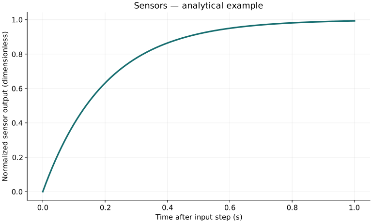
Definitions & inputs. τ time constant,x step input,y normalized output,f frequency.
One dominant storage process creates a first-order sensor model.
Solve the step response to connect settling time with dynamics.
The sinusoidal amplitude drops to 1/√2 at this frequency.
Interpretation. A fast sample rate cannot recover bandwidth removed by the sensor or analog front end.
↑ Return to definitions and contents3. Transduction examples
Definitions & inputs. R resistance,GF gauge factor,ε strain,A plate area,d gap,εd permittivity,Iph photocurrent.
Strain changes geometry and resistivity in a resistive gauge.
Electric field and stored charge produce gap-dependent capacitance.
Responsivity converts incident optical power into photocurrent.
Interpretation. Temperature, fringe fields, spectral response and saturation require additional terms in practical devices.
↑ Return to definitions and contents4. Noise and digitization
Definitions & inputs. N ADC bits,VFS span,σ independent noise,R responsivity or calibration slope.
A uniform rounding-error distribution gives quantization variance.
Independent sample variances add before averaging.
Linear uncertainty propagation combines independent small input errors.
Interpretation. Correlation introduces covariance terms, and averaging does not remove systematic bias.
↑ Return to definitions and contentsGraphical worked example
Twenty worked examples
Open a problem to see its defined inputs, assumptions, equation, numerical substitution, result, and interpretation. Values are illustrative analytical exercises.
Example 01. Linear calibration inversion
Definitions & inputs. Output y=2.5 V,offset .5 V,slope .02 V/°C.
Choose the governing model and isolate the requested quantity.
Insert the stated inputs in consistent units or the explicitly defined normalized units.
Evaluate the expression; the result uses the units shown.
Interpretation. Use this only within the calibrated temperature range.
↑ Return to definitions and contentsExample 02. Two-point sensitivity
Definitions & inputs. Output 1 V at 0 kPa and 5 V at 100 kPa.
Choose the governing model and isolate the requested quantity.
Insert the stated inputs in consistent units or the explicitly defined normalized units.
Evaluate the expression; the result uses the units shown.
Interpretation. Nonlinearity between the two calibration points remains untested.
↑ Return to definitions and contentsExample 03. Pressure from calibration
Definitions & inputs. Same slope .04 V/kPa,offset 1 V,reading 3 V.
Choose the governing model and isolate the requested quantity.
Insert the stated inputs in consistent units or the explicitly defined normalized units.
Evaluate the expression; the result uses the units shown.
Interpretation. Pressure reference must specify gauge, absolute or differential.
↑ Return to definitions and contentsExample 04. Input-referred noise
Definitions & inputs. Output standard deviation 2 mV,sensitivity .04 V/kPa.
Choose the governing model and isolate the requested quantity.
Insert the stated inputs in consistent units or the explicitly defined normalized units.
Evaluate the expression; the result uses the units shown.
Interpretation. This is noise uncertainty, not the full accuracy specification.
↑ Return to definitions and contentsExample 05. Strain-gauge resistance change
Definitions & inputs. R=120 Ω,GF=2,strain 500 microstrain.
Choose the governing model and isolate the requested quantity.
Insert the stated inputs in consistent units or the explicitly defined normalized units.
Evaluate the expression; the result uses the units shown.
Interpretation. Temperature compensation is omitted.
↑ Return to definitions and contentsExample 06. Quarter-bridge signal
Definitions & inputs. Supply 5 V,GF=2,strain 500 microstrain,small-strain bridge.
Choose the governing model and isolate the requested quantity.
Insert the stated inputs in consistent units or the explicitly defined normalized units.
Evaluate the expression; the result uses the units shown.
Interpretation. Polarity depends on which bridge arm contains the active gauge.
↑ Return to definitions and contentsExample 07. Linear RTD resistance
Definitions & inputs. R0=100 Ω at 0°C,α=.00385/K,T=50°C.
Choose the governing model and isolate the requested quantity.
Insert the stated inputs in consistent units or the explicitly defined normalized units.
Evaluate the expression; the result uses the units shown.
Interpretation. A precision platinum RTD uses a calibrated nonlinear relation over a broad range.
↑ Return to definitions and contentsExample 08. Thermocouple local voltage
Definitions & inputs. Effective local Seebeck difference 40 μV/K,junction temperature difference 100 K.
Choose the governing model and isolate the requested quantity.
Insert the stated inputs in consistent units or the explicitly defined normalized units.
Evaluate the expression; the result uses the units shown.
Interpretation. Real thermocouple tables and reference-junction compensation are required over wide ranges.
↑ Return to definitions and contentsExample 09. Ideal plate capacitance
Definitions & inputs. Vacuum gap d=.001 m,area .01 m²,ε0=8.8541878128×10⁻¹² F/m.
Choose the governing model and isolate the requested quantity.
Insert the stated inputs in consistent units or the explicitly defined normalized units.
Evaluate the expression; the result uses the units shown.
Interpretation. Fringe fields and parasitic capacitance are excluded.
↑ Return to definitions and contentsExample 10. Capacitance gap sensitivity
Definitions & inputs. Plate sensor initially 10 pF; gap reduced by 10%.
Choose the governing model and isolate the requested quantity.
Insert the stated inputs in consistent units or the explicitly defined normalized units.
Evaluate the expression; the result uses the units shown.
Interpretation. The inverse-gap law is nonlinear.
↑ Return to definitions and contentsExample 11. Photodiode current
Definitions & inputs. Responsivity .5 A/W,optical power 10 μW.
Choose the governing model and isolate the requested quantity.
Insert the stated inputs in consistent units or the explicitly defined normalized units.
Evaluate the expression; the result uses the units shown.
Interpretation. Responsivity depends on wavelength; dark current adds separately.
↑ Return to definitions and contentsExample 12. Optical round-trip ranging
Definitions & inputs. Measured delay 20 ns,c=299792458 m/s.
Choose the governing model and isolate the requested quantity.
Insert the stated inputs in consistent units or the explicitly defined normalized units.
Evaluate the expression; the result uses the units shown.
Interpretation. Divide by two because the pulse travels to the target and back.
↑ Return to definitions and contentsExample 13. Ultrasonic range
Definitions & inputs. Round-trip delay .01 s,sound speed 343 m/s.
Choose the governing model and isolate the requested quantity.
Insert the stated inputs in consistent units or the explicitly defined normalized units.
Evaluate the expression; the result uses the units shown.
Interpretation. Temperature, humidity and target geometry affect the return.
↑ Return to definitions and contentsExample 14. Encoder angle
Definitions & inputs. 100 counts with 4000 resolved counts/revolution.
Choose the governing model and isolate the requested quantity.
Insert the stated inputs in consistent units or the explicitly defined normalized units.
Evaluate the expression; the result uses the units shown.
Interpretation. Resolved counts already include quadrature decoding if used.
↑ Return to definitions and contentsExample 15. Accelerometer calibration
Definitions & inputs. Output change .3 V,sensitivity .3 V per g.
Choose the governing model and isolate the requested quantity.
Insert the stated inputs in consistent units or the explicitly defined normalized units.
Evaluate the expression; the result uses the units shown.
Interpretation. An accelerometer measures specific force; orientation and gravity must be distinguished.
↑ Return to definitions and contentsExample 16. Gyroscope angle drift
Definitions & inputs. Constant bias .1 degree/s over 60 s.
Choose the governing model and isolate the requested quantity.
Insert the stated inputs in consistent units or the explicitly defined normalized units.
Evaluate the expression; the result uses the units shown.
Interpretation. Bias integration can dominate long-duration inertial orientation.
↑ Return to definitions and contentsExample 17. First-order 90% response
Definitions & inputs. τ=.2 s.
Choose the governing model and isolate the requested quantity.
Insert the stated inputs in consistent units or the explicitly defined normalized units.
Evaluate the expression; the result uses the units shown.
Interpretation. The sensor response bandwidth is independent of the digital display refresh rate.
↑ Return to definitions and contentsExample 18. ADC voltage resolution
Definitions & inputs. 12 bits,span 4.096 V.
Choose the governing model and isolate the requested quantity.
Insert the stated inputs in consistent units or the explicitly defined normalized units.
Evaluate the expression; the result uses the units shown.
Interpretation. A millivolt code step does not imply millivolt absolute accuracy.
↑ Return to definitions and contentsExample 19. Averaged random uncertainty
Definitions & inputs. Independent standard deviation 2 units per sample,n=100.
Choose the governing model and isolate the requested quantity.
Insert the stated inputs in consistent units or the explicitly defined normalized units.
Evaluate the expression; the result uses the units shown.
Interpretation. Correlated drift and fixed calibration bias do not average away this way.
↑ Return to definitions and contentsExample 20. Independent uncertainty combination
Definitions & inputs. Two independent standard uncertainty contributions .3 and .4 units.
Choose the governing model and isolate the requested quantity.
Insert the stated inputs in consistent units or the explicitly defined normalized units.
Evaluate the expression; the result uses the units shown.
Interpretation. This is a combined standard uncertainty, not an automatically 95% expanded interval.
↑ Return to definitions and contentsSymbols and units
Each derivation and problem defines its own symbols and inputs. Symbols may be reused with different meanings in other subjects. Keep units consistent, retain sufficient precision during calculation, and apply the stated validity limits.
THE SENSORS COMMUNITY
Cumulative visitor map
Distinct daily visits, cumulative
Counting since 2026-09-25 (UTC). As on To the Infinity, one IP address counts once per UTC day; this is not a count of registered accounts or unique people across all time. Shared networks and automated traffic can affect totals.
Cumulative location countYour approximate current location
Your approximate current location: Columbus, US. This blue marker is shown only in your response.
Locations are approximate IP-derived city/region estimates, never GPS. Public markers require at least three cumulative daily visits. Sensors stores aggregate locations and short-lived keyed daily identifiers outside the public site, not raw IP addresses. Map boundaries are for orientation, not a statement of jurisdiction.
Visitor locations & map sources
- New York, US — 7 cumulative daily visits
- Tracy, US — 7 cumulative daily visits
- Los Angeles, US — 5 cumulative daily visits
- Santa Clara, US — 4 cumulative daily visits
- London, GB — 3 cumulative daily visits
- Council Bluffs, US — 3 cumulative daily visits
- Mountain View, US — 3 cumulative daily visits
Basemap: World Atlas, derived from Natural Earth public-domain map data. IP geolocation uses the same local database as To the Infinity.