Spaceflight trajectory calculation

Trajectory atlas: what has flown, and what remains a concept

Flown status refers to a family, not every possible member. This guide indexes the main classes; follow the mission archives for individual dates, flight paths and records.

Earth-bound and Earth orbit

Ballistic suborbital arcs; circular and elliptical LEO; high-inclination and polar orbits; rendezvous and phasing; geosynchronous/GEO, Molniya/Tundra, sun-synchronous and disposal orbits. Humans have flown suborbital and low Earth trajectories, including high-apogee and polar LEO. GEO and the other high operational orbit families have been robotic.

Lunar and libration-point

Translunar injection, lunar flyby/free return, lunar capture and landing/ascent, Earth return; halo/Lissajous, DRO, NRHO and low-energy transfers. Apollo flew lunar orbit and landing routes; Apollo13 returned after a corrected lunar flyby. ArtemisII completed its crewed lunar flyby in April2026. Robotic examples include ArtemisI’s DRO, CAPSTONE’s NRHO and JWST’s Sun–EarthL2 halo orbit.

Interplanetary

Direct Lambert transfers, Hohmann-like transfers, resonant gravity-assist tours, low-thrust spirals, capture, aerobraking, landing and sample return. Voyager used planetary assists; Dawn used ion propulsion; Mars orbiters have used aerobraking. Bi-elliptic transfers are an analytical family; cyclers, solar Oberth interstellar departures and aerocapture need mission-specific status, not an assumption that every concept has flown.

Solar escape and interstellar

Pioneer10/11, Voyager1/2 and New Horizons follow solar escape paths. Both Voyagers have crossed the heliopause. None has reached another star, and no human has traveled on an interplanetary or interstellar mission. A Proxima flyby could conceptually use a high-speed probe; arrival at rest adds a separate braking requirement.

Human-flown trajectory families and program records

• Ballistic suborbital: Mercury-Redstone, New Shepard and crewed launch-abort returns; winged suborbital: X-15, SpaceShipOne and SpaceShipTwo. Space-flight counting differs between the80km and100km conventions.
• Low Earth orbit and rendezvous: Vostok, Voskhod, Mercury-Atlas, Gemini, Apollo7/9, Soyuz, Shenzhou, Space Shuttle, Crew Dragon and Starliner’s2024 crewed outbound test flight; stations include Salyut, Skylab, Mir, ISS and Tiangong. Starliner’s return on that test was uncrewed.
• High-apogee/polar LEO: Gemini11, Polaris Dawn (1408.1km peak altitude) and Fram2’s2025 polar mission broaden the crewed LEO family; they are not GEO flights.
• Lunar orbit: Apollo8,10,11,12,14,15,16,17. Lunar landing/ascent: Apollo11,12,14,15,16,17. Lunar flyby/return: Apollo13 and ArtemisII. Apollo paths involved mission-specific corrections; “free return” does not mean no maneuvers at all.

Records: NASA human-spaceflight history · Apollo mission archive · ArtemisII · Chinese human-spaceflight missions · Polaris Dawn · Fram2 · Voyager and solar escape. Historical status checked24September2026.

1. State vectors, conics and time of flight

Definitions & inputs. r and v are relative position and velocity, μ gravitational parameter, h specific angular momentum, ε specific energy, e eccentricity, a semimajor axis, E eccentric anomaly.

1. Integrate Newton’s equation; energy and angular momentum are its two-body invariants.

   $$\ddot{\mathbf r}=-\mu\mathbf r/r^3,\quad\epsilon=v^2/2-\mu/r,\quad\mathbf h=\mathbf r\times\mathbf v$$

2. Recover the conic from a state vector. The parabolic limit has ε=0 and no finite a.

   $$\mathbf e=\frac{\mathbf v\times\mathbf h}{\mu}-\frac{\mathbf r}{r},\quad a=-\mu/(2\epsilon)$$

3. e<1 gives an ellipse, e=1 a parabola and e>1 a hyperbola. These are shapes, not complete dated flight plans.

   $$r(\nu)=\frac{h^2/\mu}{1+e\cos\nu},\quad v^2=\mu(2/r-1/a)$$

4. For an ellipse, solve Kepler’s equation to map position to time. A uniform true-angle sampling is not uniform time.

   $$n=\sqrt{\mu/a^3},\quad n(t-t_p)=E-e\sin E$$

Worked example: Circular state and elapsed orbital phase

μ=398600.4418 km³/s², r=7000 km, circular equatorial orbit, start at x=r with velocity along positive y.

1. Choose the speed that balances radial gravity.

   $$v_c=\sqrt{398600.4418/7000}=7.54605\ \mathrm{km/s}$$

2. Substitute circular speed in the energy and eccentricity formulas.

   $$\epsilon=-\mu/(2r)=-28.47146\ \mathrm{km^2/s^2},\quad e=0$$

3. A quarter orbit advances both mean and true anomaly by π/2 in the circular special case.

   $$\Delta t=\pi/[2\sqrt{\mu/r^3}]=1457.129\ \mathrm s$$

Interpretation. Specify inertial versus rotating coordinates, units, central body, epoch, time scale and frame orientation before comparing state vectors. Hyperbolic and parabolic timing require their corresponding anomaly equations. Worked-example interpretation: The state, epoch and elapsed time determine the endpoint; radius by itself would not.

• NASA — Basics of Space Flight: orbital mechanics ↗

2. Earth-orbit and interplanetary Hohmann transfers

Definitions & inputs. r1<r2 are coplanar circular radii around the same primary, at transfer semimajor axis, n2 final mean motion, φ target angular lead at departure.

1. Choose an ellipse tangent to both circular orbits and evaluate departure speed.

   $$a_t=(r_1+r_2)/2,\quad v_{t1}=\sqrt{\mu(2/r_1-1/a_t)}$$

2. Subtract the circular endpoint speeds using the correct departure and arrival directions.

   $$\Delta v_1=v_{t1}-\sqrt{\mu/r_1},\quad\Delta v_2=\sqrt{\mu/r_2}-\sqrt{\mu(2/r_2-1/a_t)}$$

3. The craft travels half an ellipse while the target advances toward the opposite endpoint.

   $$t_H=\pi\sqrt{a_t^3/\mu},\quad \phi=\pi-\sqrt{\mu/r_2^3}\,t_H$$

4. At a planetary encounter use a vector difference; a scalar speed difference is sufficient only in the collinear ideal example.

   $$v_\infty=|\mathbf v_{transfer}-\mathbf v_{planet}|,\quad C_3=v_\infty^2$$

5. A patched-conic energy balance converts hyperbolic excess speed into a tangential parking-orbit departure impulse.

   $$\Delta v_{escape}=\sqrt{2\mu_E/r_p+v_\infty^2}-\sqrt{\mu_E/r_p}$$

Worked example: Two burns from 7000 km to 14000 km radius

Use μ=398600.4418 km³/s², circular coplanar endpoints and instantaneous tangential burns.

1. Tangency fixes the transfer ellipse’s apsides and semimajor axis.

   $$a_t=(7000+14000)/2=10500\ \mathrm{km}$$

2. Subtract endpoint circular and transfer speeds with the proper sign at each burn.

   $$\Delta v_1=1.16738\ \mathrm{km/s},\quad\Delta v_2=0.979150\ \mathrm{km/s}$$

3. Sum burn magnitudes; coast time is half the transfer period.

   $$\Delta v_{total}=2.14653\ \mathrm{km/s},\quad t_H=\pi\sqrt{10500^3/\mu}=5353.834\ \mathrm s$$

Interpretation. A bi-elliptic transfer can reduce impulsive Δv for some radius ratios at the cost of longer flight time; a pure plane change costs2v sin(Δi/2). Finite thrust and combined plane changes require a different optimization. Worked-example interpretation: Arrival at the correct radius does not guarantee rendezvous: target phase must also match the transfer time.

• NASA — Basics of Space Flight: orbital mechanics ↗

3. Lunar, low-energy, gravity-assist and low-thrust trajectories

Definitions & inputs. ri are attracting-body positions, T thrust, m spacecraft mass, vin∞ and vout∞ incoming and outgoing planet-relative asymptotic velocities.

1. Integrate gravity, thrust and appropriate perturbations rather than attaching unrelated Kepler arcs blindly.

   $$\ddot{\mathbf r}=\sum_i\mu_i\frac{\mathbf r_i-\mathbf r}{|\mathbf r_i-\mathbf r|^3}+\mathbf T/m+\mathbf a_{other}$$

2. A gravity assist rotates the planet-relative velocity; adding the moving planet velocity changes heliocentric energy.

   $$\mathbf v_{helio,in}=\mathbf v_p+\mathbf v_{\infty,in},\quad\mathbf v_{helio,out}=\mathbf v_p+\mathbf v_{\infty,out}$$

3. An unpowered point-mass flyby conserves planet-relative excess speed; periapsis and excess speed determine deflection.

   $$|\mathbf v_{\infty,in}|=|\mathbf v_{\infty,out}|,\quad\delta=2\arcsin\!\left[\frac1{1+r_pv_\infty^2/\mu_p}\right]$$

4. Solve a boundary-value transfer for specified endpoints and duration; multiple branches and revolutions can exist.

   $$\mathrm{Lambert}:\quad(\mathbf r_1,\mathbf r_2,\Delta t,\mu)\longmapsto(\mathbf v_1,\mathbf v_2)$$

Worked example: Patched-conic departure from a parking orbit

Parking radius rp=7000 km, Earth μ=398600.4418 km³/s² and required planet-relative excess speed v∞=3 km/s.

1. Express the departure requirement as characteristic energy.

   $$C_3=v_\infty^2=9\ \mathrm{km^2/s^2}$$

2. Use conservation of planet-relative hyperbolic energy.

   $$v_{peri}=\sqrt{2\mu/r_p+v_\infty^2}=11.08539\ \mathrm{km/s}$$

3. Subtract the circular parking speed for a tangential injection at periapsis.

   $$\Delta v=11.08539-7.54605=3.53933\ \mathrm{km/s}$$

Interpretation. Lunar free-return paths, halo/Lissajous orbits, distant retrograde orbits (DRO), near-rectilinear halo orbits (NRHO), and manifold transfers use multibody dynamics. Low-thrust spirals continuously change energy; aerobraking dissipates it over repeated atmospheric passes. Aerocapture is a distinct single-pass capture concept. Perturbations, corrections, navigation uncertainty and station keeping remain essential. Worked-example interpretation: This excludes launch, finite-burn losses and arrival capture; it illustrates the interface between planetary and heliocentric arcs.

• JPL Horizons — reference frames, ephemerides and state vectors ↗

4. Nearest-star route: cruise, proper time and stopping

Definitions & inputs. Proxima Centauri is the nearest star beyond the Sun. D=4.25ly is a rounded exercise distance; β=v/c, γ=(1−β²)⁻¹/², τ ship proper time. One light-year is c times one Julian year.

1. Earth-frame travel time differs from time on the coasting ship.

   $$t_E=D/(\beta c),\quad\tau=t_E\sqrt{1-\beta^2}$$

2. A tenth of light speed still takes more than four decades at the assumed distance.

   $$\beta=0.1:\quad t_E=42.5\,\mathrm{yr},\quad\tau=42.28697\,\mathrm{yr}$$

3. Kinetic energy per kilogram is a lower-level energy quantity, not a total propulsion budget. Signals also take years.

   $$K/m=(\gamma-1)c^2,\quad t_{light}=D/c=4.25\,\mathrm{yr}$$

4. For a separate ideal profile, accelerate at constant proper acceleration a halfway, then reverse acceleration to arrive at rest. Integrate relativistic constant-proper-acceleration motion on each half.

   $$u=1+\frac{aD}{2c^2},\quad t_E=\frac{2c}{a}\sqrt{u^2-1},\quad\tau=\frac{2c}{a}\operatorname{arcosh}u$$

5. The midpoint speed remains below c. Maintaining such acceleration over interstellar distances is not an established propulsion capability.

   $$v_{max}=c\sqrt{1-u^{-2}}$$

6. To derive the accelerated profile, introduce rapidity χ. Constant proper acceleration makes rapidity increase linearly with onboard proper time, starting from rest.

   $$\chi=\operatorname{artanh}(v/c),\quad d\chi/d\tau=a/c,\quad dt/d\tau=\cosh\chi$$

7. Integrate dt/dτ and dx/dτ=c sinh χ from rest at the origin; the integration constants enforce t=x=0 initially.

   $$\chi=a\tau/c,\quad t(\tau)=\frac ca\sinh(a\tau/c),\quad x(\tau)=\frac{c^2}{a}[\cosh(a\tau/c)-1]$$

8. Set the half-trip distance and solve for half-trip proper time. Doubling the symmetric accelerating and decelerating halves gives the formulas above; the midpoint Lorentz factor is u.

   $$x(\tau_{half})=D/2\quad\Longrightarrow\quad\cosh(a\tau_{half}/c)=1+aD/(2c^2)=u$$

Worked example: Interstellar cruise and a distinct accelerated profile

Use a fixed distance D=4.25 light-years. First coast at β=0.1 with instantaneous start/stop omitted; then separately use proper acceleration a=9.80665 m/s² halfway and reverse it halfway. One Julian year is 31557600 s.

1. The coasting ship’s proper time is shorter by the Lorentz factor.

   $$t_E=4.25/0.1=42.5\ \mathrm{yr},\quad\tau=42.5\sqrt{0.99}=42.28697\ \mathrm{yr}$$

2. For the separate accelerating-and-braking model, convert light-years to metres before forming dimensionless u.

   $$u=1+\frac{aD}{2c^2}\simeq3.19361,\quad v_{max}/c=\sqrt{1-u^{-2}}\simeq0.94971$$

3. Evaluate the two-half-trip formulas; arcosh(u)=ln(u+√(u²−1)). These times describe a different profile from the 0.1c coast.

   $$t_E\simeq5.876\ \mathrm{yr},\quad\tau\simeq3.54325\ \mathrm{yr}$$

Interpretation. A flyby and a rendezvous are different missions: arrival at rest needs deceleration. Chemical, electric, nuclear, fusion, antimatter and beam-driven concepts have different energy and propellant budgets. No spacecraft has reached another star; solar-system escape and crossing the heliopause do not mean stellar arrival. Worked-example interpretation: The constant-proper-acceleration scenario is a kinematic thought experiment, not an available propulsion system; target motion and energy supply are omitted.

• NASA Hubble — Proxima Centauri ↗

5. Derive the conic equation from Newton’s law

Definitions & inputs. r is distance from the central body, μ gravitational parameter, h specific angular-momentum magnitude, ν true anomaly, u=1/r, ε specific energy, p semilatus rectum.

1. Take the cross product with position. A central force exerts no torque, so angular momentum has fixed direction and the orbit lies in one plane.

   $$\ddot{\mathbf r}=-\mu\mathbf r/r^3,\qquad\dot{\mathbf h}=\mathbf r\times\ddot{\mathbf r}=0$$

2. Dot the equation of motion with velocity and integrate. Kinetic plus gravitational potential energy per unit mass is constant.

   $$\mathbf v\cdot\ddot{\mathbf r}=\frac{d}{dt}\frac{v^2}{2}=-\frac{\mu\dot r}{r^2}\quad\Longrightarrow\quad\epsilon=\frac{v^2}{2}-\frac{\mu}{r}$$

3. Use conserved angular momentum to change the independent variable from time to angle.

   $$h=r^2\dot\nu,\quad\dot r=-h\frac{du}{d\nu},\quad\ddot r=-h^2u^2\frac{d^2u}{d\nu^2}$$

4. Insert the reciprocal-radius derivatives into the radial acceleration equation. The nonlinear radial motion becomes a linear forced equation in angle.

   $$\ddot r-r\dot\nu^2=-\mu/r^2\quad\Longrightarrow\quad u^{\prime\prime}+u=\mu/h^2$$

5. Solve the linear equation and choose periapsis as ν=0; the homogeneous amplitude defines eccentricity.

   $$u=\frac{\mu}{h^2}(1+e\cos\nu),\quad r=\frac{p}{1+e\cos\nu},\quad p=\frac{h^2}{\mu}$$

6. Substitute radial and transverse velocities into the energy integral. Ellipses have ε<0, parabolas ε=0 and hyperbolas ε>0; a is negative on a hyperbola.

   $$e^2=1+\frac{2\epsilon h^2}{\mu^2},\quad\epsilon=-\frac{\mu}{2a},\quad v^2=\mu(2/r-1/a)$$

Worked example: Recover an ellipse from a tangential state

At r=7000 km, radial speed is zero and transverse speed is 8 km/s; μ=398600.4418 km³/s². This speed exceeds circular speed but is below escape speed.

1. Use the velocity perpendicular to radius for angular momentum.

   $$h=7000(8)=56000\ \mathrm{km^2/s},\quad\epsilon=8^2/2-398600.4418/7000=-24.9429\ \mathrm{km^2/s^2}$$

2. At this tangential, faster-than-circular state the starting point is periapsis.

   $$a=-\mu/(2\epsilon)=7990.253\ \mathrm{km},\quad e=\frac{7000(8)^2}{\mu}-1=0.123933$$

3. Recover the opposite apsis and check that rp=a(1−e).

   $$r_a=2a-r_p=8980.505\ \mathrm{km}$$

Interpretation. An orbit shape does not fix when the spacecraft reaches a point; time evolution requires a separate anomaly equation. Worked-example interpretation: The 7000 km input is radius from the centre, not altitude. The bound-energy sign independently confirms the ellipse.

• MIT OpenCourseWare — Astrodynamics: derivations and lecture notes ↗

6. Derive Kepler’s equation and solve it iteratively

Definitions & inputs. a semimajor axis, e eccentricity, E eccentric anomaly, M mean anomaly, n mean motion, tp periapsis epoch, ν true anomaly.

1. Parameterize the ellipse with its focus at the origin. E is an auxiliary angle, not the geometric angle at the focus.

   $$x=a(\cos E-e),\quad y=a\sqrt{1-e^2}\sin E,\quad r=a(1-e\cos E)$$

2. Compute swept-area rate from one half of x dy minus y dx. Angular-momentum conservation fixes equal areas in equal times.

   $$\frac{dA}{dE}=\frac12a^2\sqrt{1-e^2}(1-e\cos E),\quad\frac{dA}{dt}=h/2$$

3. Divide the two area derivatives, then insert h²=μa(1−e²).

   $$\frac{dt}{dE}=\frac{1-e\cos E}{n},\quad n=\sqrt{\mu/a^3}$$

4. Integrate from periapsis, where E=0. This relation is implicit in E.

   $$M=n(t-t_p)=E-e\sin E$$

5. Newton’s method subtracts residual divided by local slope. Near e=1 and periapsis the slope becomes small; use a safeguarded bracket or robust solver.

   $$F(E)=E-e\sin E-M,\quad E_{k+1}=E_k-\frac{F(E_k)}{1-e\cos E_k}$$

6. A two-argument arctangent preserves the quadrant. Check both the equation residual and the change in E before stopping.

   $$\nu=\operatorname{atan2}(\sqrt{1-e^2}\sin E,\cos E-e)$$

Worked example: Propagate to mean anomaly 1 radian

a=10000 km, e=0.2, M=1 rad, μ=398600.4418 km³/s²; start Newton iteration at E0=M.

1. Evaluate residual and derivative at the starting guess.

   $$E_1=1-\frac{1-0.2\sin1-1}{1-0.2\cos1}=1.188683$$

2. Further iterations give the root. The time follows from M/n independently of the root solution.

   $$E\simeq1.185324\ \mathrm{rad},\quad t-t_p=1/\sqrt{398600.4418/10000^3}=1583.912\ \mathrm s$$

3. Use the solved eccentric anomaly to recover radius; rounded values leave a small residual.

   $$r=10000(1-0.2\cos1.185324)=9248.007\ \mathrm{km}$$

Interpretation. Uniform sampling in E or ν does not produce uniform time intervals. Mean anomaly advances uniformly only in the unperturbed model. Worked-example interpretation: At the same mean anomaly, a circular orbit would stay at 10000 km; eccentric geometry changes the position and speed.

• MIT OpenCourseWare — Astrodynamics: derivations and lecture notes ↗

7. Hyperbolic and parabolic time of flight

Definitions & inputs. A=−a>0 is hyperbolic semimajor-axis magnitude, H hyperbolic anomaly, nh hyperbolic mean-motion scale, q parabolic periapsis radius and D=tan(ν/2).

1. Positive orbital energy gives an asymptotic excess speed. The hyperbola uses e>1 and a negative signed semimajor axis.

   $$\epsilon=\frac{\mu}{2A}=\frac{v_\infty^2}{2},\quad r=A(e\cosh H-1)$$

2. Hyperbolic area integration gives the time relation, analogous to the elliptic Kepler equation.

   $$n_h=\sqrt{\mu/A^3},\qquad n_h(t-t_p)=e\sinh H-H$$

3. Differentiate the hyperbolic time residual to obtain a Newton update. Large anomalies require care with overflow and initial guesses.

   $$H_{k+1}=H_k-\frac{e\sinh H_k-H_k-n_h(t-t_p)}{e\cosh H_k-1}$$

4. For a parabola, use p=2q and the half-angle identity for the conic radius.

   $$e=1:\quad r=q(1+D^2),\quad h=\sqrt{2\mu q}$$

5. Substitute dν=2 dD/(1+D²) into the equal-area time relation.

   $$dt=\frac{r^2}{h}\,d\nu=\sqrt{\frac{2q^3}{\mu}}(1+D^2)\,dD$$

6. Integrating gives Barker’s equation; it remains finite at parabolic energy, where elliptic a diverges.

   $$t-t_p=\sqrt{\frac{2q^3}{\mu}}\left(D+\frac{D^3}{3}\right)$$

Worked example: A parabolic Earth escape at 90 degrees past periapsis

q=7000 km, μ=398600.4418 km³/s² and ν=90 degrees. This is an exact escape-energy idealization.

1. Use the half-angle variable to obtain radius.

   $$D=\tan45^\circ=1,\quad r=7000(1+1)=14000\ \mathrm{km}$$

2. Evaluate the finite parabolic time of flight.

   $$t-t_p=\sqrt{2(7000)^3/398600.4418}(1+1/3)=1749.170\ \mathrm s$$

3. Parabolic energy is zero, so speed at every radius equals the local two-body escape speed.

   $$v=\sqrt{2\mu/r}=7.54605\ \mathrm{km/s}$$

Interpretation. Near-parabolic motion is numerically awkward if formulas subtract large nearly equal quantities; universal-variable propagators can bridge conic types. Worked-example interpretation: Reaching 14000 km radius takes about 29.15 minutes after periapsis; a finite-radius speed is not v∞.

• MIT OpenCourseWare — Astrodynamics: derivations and lecture notes ↗

8. Transform positions and velocities between frames

Definitions & inputs. Q(t) rotates body-fixed coordinates into inertial coordinates, Ω is frame angular velocity in inertial axes, rO and vO describe the moving origin.

1. Translate the origin and rotate the components. A position vector is incomplete without both its origin and axis definition.

   $$\mathbf r_I=\mathbf r_O+Q\mathbf r_F$$

2. Differentiate the entire position relation. Rotating the velocity components alone omits the time derivative of the axes.

   $$\mathbf v_I=\mathbf v_O+Q\mathbf v_F+\dot Q\mathbf r_F$$

3. The missing velocity is the transport velocity due to frame rotation.

   $$\dot Q\mathbf r_F=\boldsymbol\Omega\times(Q\mathbf r_F)$$

4. A second derivative yields Coriolis, Euler and centripetal terms. All displayed cross products are expressed in inertial axes.

   $$\mathbf a_I=\mathbf a_O+Q\mathbf a_F+2\boldsymbol\Omega\times Q\mathbf v_F+\dot{\boldsymbol\Omega}\times Q\mathbf r_F+\boldsymbol\Omega\times(\boldsymbol\Omega\times Q\mathbf r_F)$$

5. For Earth-centred, nonrotating relative coordinates, subtract the third body’s acceleration of Earth. rB is measured from Earth; the bracket is the direct plus indirect third-body contribution.

   $$\ddot{\mathbf r}=-\frac{\mu_E\mathbf r}{r^3}+\mu_B\left[\frac{\mathbf r_B-\mathbf r}{|\mathbf r_B-\mathbf r|^3}-\frac{\mathbf r_B}{r_B^3}\right]$$

Worked example: A fixed point on the equator is moving inertially

Take RE=6371 km and Earth angular rate Ω=7.2921159×10⁻⁵ rad/s. At the selected instant Q is the identity, position is (RE,0,0), and body-fixed velocity is zero.

1. Use Ω along the positive z axis and evaluate the cross product.

   $$\mathbf v_I=(0,\Omega R_E,0),\quad\Omega R_E=0.464581\ \mathrm{km/s}$$

2. For uniform rotation the acceleration points toward the spin axis.

   $$|\mathbf a_I|=\Omega^2R_E=3.38778\times10^{-5}\ \mathrm{km/s^2}$$

3. This is arc length travelled in one minute, illustrating the error scale from omitting transport velocity.

   $$\Delta s\simeq v_I(60)=27.8748\ \mathrm{km}$$

Interpretation. A complete state exchange also records epoch, time scale, units, central body and whether apparent light-time corrections were applied. Worked-example interpretation: For operational transformations use epoch-matched Earth orientation and validated frame kernels.

• NASA/JPL NAIF — Reference frames and state transformations ↗

9. Lambert targeting and departure-window searches

Definitions & inputs. r1 and r2 are endpoint position vectors at times t1 and t2, Δt flight time; f,g and their time derivatives are Lagrange propagation coefficients.

1. Two-body motion stays in the initial state plane, so endpoint states can be written as linear combinations of initial position and velocity with scalar dynamical coefficients.

   $$\mathbf r_2=f\mathbf r_1+g\mathbf v_1,\quad\mathbf v_2=\dot f\mathbf r_1+\dot g\mathbf v_1$$

2. Once a Lambert solver determines time-consistent coefficients, solve for departure and arrival velocities. These formulas require g≠0; collinear geometries need special handling.

   $$\mathbf v_1=\frac{\mathbf r_2-f\mathbf r_1}{g},\quad\mathbf v_2=\dot f\mathbf r_1+\dot g\mathbf v_1$$

3. The Lagrange coefficient identity follows from angular-momentum conservation and is a useful internal check, though it does not alone prove endpoint accuracy.

   $$f\dot g-\dot f g=1$$

4. Subtract the departure planet’s velocity in the same heliocentric frame. Arrival excess speed is obtained by the corresponding arrival subtraction.

   $$\mathbf v_{\infty,dep}=\mathbf v_1-\mathbf v_{planet}(t_1),\quad C_3=|\mathbf v_{\infty,dep}|^2$$

5. A departure/arrival date grid can visualize one chosen screening objective. Weights, flight time, launch asymptote and capture constraints must be explicit; the lowest C3 is not always the best mission.

   $$J(t_1,t_2)=w_1C_3+w_2|\mathbf v_{\infty,arr}|^2$$

6. Independently propagate the returned initial state for the requested duration and check terminal position and branch. Refine shortlisted solutions with ephemerides and perturbations.

   $$\delta\mathbf r=\mathbf r_{prop}(t_2)-\mathbf r_2$$

Worked example: A quarter-circle Lambert benchmark

μ=398600.4418 km³/s², r=7000 km, r1=(r,0,0), r2=(0,r,0), prograde transfer. Choose Δt equal to one quarter of the circular period.

1. The selected flight time admits the obvious circular solution on this branch.

   $$n=\sqrt{\mu/r^3}=0.00107801\ \mathrm{s^{-1}},\quad\Delta t=\pi/(2n)=1457.129\ \mathrm s$$

2. For a circular reference arc, the coefficients reduce to sine and cosine.

   $$f=\cos(n\Delta t)=0,\quad g=\sin(n\Delta t)/n=927.637\ \mathrm s$$

3. The departure velocity is r2/g; the arrival direction has turned by 90 degrees. Substitution into propagation recovers both endpoints.

   $$\mathbf v_1=(0,7.54605,0),\quad\mathbf v_2=(-7.54605,0,0)\ \mathrm{km/s}$$

Interpretation. This section explains targeting and gives a solvable benchmark; it does not present a general Lambert solver or claim a mission launch window. Worked-example interpretation: Changing Δt while keeping the same endpoints generally destroys the circular solution and requires solving the boundary-value problem.

• MIT OpenCourseWare — Astrodynamics: derivations and lecture notes ↗

10. Derive gravity-assist bending and energy exchange

Definitions & inputs. vp planet heliocentric velocity, v∞ planet-relative asymptotic speed, rp flyby periapsis radius, μp planet gravitational parameter, δ asymptotic turn angle, b impact parameter.

1. The hyperbola’s periapsis is A(e−1); substitute its positive-energy semimajor-axis magnitude.

   $$\epsilon_p=v_\infty^2/2,\quad A=\mu_p/v_\infty^2,\quad e=1+r_pv_\infty^2/\mu_p$$

2. At infinity the conic denominator vanishes. Asymptote geometry then gives the angle between incoming and outgoing velocity vectors.

   $$1+e\cos\nu_\infty=0,\quad\delta=2\arcsin(1/e)$$

3. Conserve angular momentum and use periapsis energy to connect an incoming impact parameter to closest approach.

   $$h=bv_\infty=r_pv_{peri},\quad b^2=r_p^2+2\mu_pr_p/v_\infty^2$$

4. A purely gravitational unpowered flyby preserves planet-relative asymptotic speed while rotating its direction.

   $$|\mathbf v_{\infty,out}|=|\mathbf v_{\infty,in}|,\quad\mathbf v_{helio}=\mathbf v_p+\mathbf v_\infty$$

5. Expand the heliocentric kinetic energies before and after. The equal v∞² terms cancel; orientation relative to planet motion determines gain or loss.

   $$\Delta\epsilon_{helio}=\mathbf v_p\cdot(\mathbf v_{\infty,out}-\mathbf v_{\infty,in})$$

6. The vector difference is a chord of a velocity-space circle. The dot product is largest when that chord aligns with planet velocity; mission geometry may prevent that alignment.

   $$|\Delta\epsilon_{helio}|\leq2v_pv_\infty\sin(\delta/2)$$

Worked example: Hypothetical Earth flyby

μp=398600.4418 km³/s², rp=7000 km and v∞=5 km/s; use vp=29.78 km/s only for an orientation-independent upper bound.

1. Find eccentricity from closest approach and excess speed.

   $$e=1+7000(5)^2/398600.4418=1.439036$$

2. Convert the asymptotic turn angle to degrees only after evaluating the inverse sine.

   $$\delta=2\arcsin(1/e)\simeq88.04^\circ$$

3. Use sin(δ/2)=1/e to evaluate the bound; this is not an achieved mission energy gain.

   $$|\Delta\epsilon_{helio}|\leq2(29.78)(5)/1.439036\simeq206.944\ \mathrm{km^2/s^2}$$

Interpretation. A gravity assist does not create energy in the planet frame. The heliocentric spacecraft exchanges a tiny amount of energy and momentum with the moving planet. Worked-example interpretation: The approach direction and B-plane orientation decide the actual sign and magnitude of energy change.

• MIT OpenCourseWare — Astrodynamics: derivations and lecture notes ↗

11. Low-thrust spirals, mass flow and power limits

Definitions & inputs. at is tangential acceleration, a orbit semimajor axis, T thrust magnitude, m instantaneous mass, ve exhaust speed, P electrical input and η thruster efficiency.

1. Dot the thrust acceleration with velocity. Only the component along motion changes orbital energy instantaneously.

   $$\dot\epsilon=\mathbf v\cdot\mathbf a_T\simeq\sqrt{\mu/a}\,a_t$$

2. Differentiate energy with respect to semimajor axis and equate it to thrust work per unit mass.

   $$\epsilon=-\mu/(2a)\quad\Longrightarrow\quad\dot a=2a^{3/2}a_t/\sqrt\mu$$

3. Separate variables for constant tangential acceleration.

   $$\int_{a_1}^{a_2}a^{-3/2}\,da=\frac{2a_t}{\sqrt\mu}\int_0^{t_f}dt$$

4. Integrate to get an approximate spiral duration. The positive thrust integral equals the decrease in circular speed even while orbital energy increases.

   $$t_f=\frac{\sqrt\mu}{a_t}\left(\frac{1}{\sqrt{a_1}}-\frac{1}{\sqrt{a_2}}\right),\quad\int_0^{t_f}a_tdt=v_{c1}-v_{c2}$$

5. Mass conservation and jet kinetic power connect propellant flow, exhaust speed and thrust. Higher exhaust speed reduces thrust at fixed electrical power.

   $$\dot m=-T/v_e,\quad\eta P=\tfrac12|\dot m|v_e^2\quad\Longrightarrow\quad T=2\eta P/v_e$$

6. For finite burns integrate position, velocity and mass together, with steering, eclipse outages and power availability specified.

   $$\ddot{\mathbf r}=-\mu\mathbf r/r^3+\frac{T}{m}\hat{\mathbf u},\quad\dot m=-\frac{T}{I_{sp}g_0}$$

Worked example: Slowly raise a circular Earth orbit

a1=7000000 m, a2=8000000 m, μ=3.986004418×10¹⁴ m³/s² and at=0.0001 m/s² throughout.

1. Compute the thrust integral for this approximate spiral.

   $$v_{c1}-v_{c2}=\sqrt{\mu/7000000}-\sqrt{\mu/8000000}=487.367\ \mathrm{m/s}$$

2. Divide by the prescribed continuous acceleration; eclipse interruptions would lengthen elapsed time.

   $$t_f=487.367/10^{-4}\simeq4.87367\times10^6\ \mathrm s\simeq56.408\ \mathrm{day}$$

3. At an instantaneous mass of 100 kg, this acceleration needs 10 mN; keeping acceleration fixed requires throttling as mass changes.

   $$T=ma_t=100(10^{-4})=0.010\ \mathrm N$$

Interpretation. An impulsive Δv budget alone cannot determine low-thrust flight time or steering; the circular-spiral result is a limited benchmark. Worked-example interpretation: The vehicle slows in circular speed while gaining potential energy; this is why speed change alone can mislead orbital reasoning.

• MIT OpenCourseWare — Astrodynamics: derivations and lecture notes ↗

12. J2 precession and atmospheric orbital decay

Definitions & inputs. J2 dimensionless oblateness coefficient, RE equatorial reference radius associated with J2, p=a(1−e²), i inclination, Ω ascending node, ρ atmospheric density, CD drag coefficient, A/m area-to-mass ratio.

1. The quadrupole term describes the leading axisymmetric deviation from a point-mass potential; φ is geocentric latitude.

   $$U=-\frac{\mu}{r}\left[1-J_2\left(\frac{R_E}{r}\right)^2\frac{3\sin^2\varphi-1}{2}\right]$$

2. Orbit averaging the quadrupole torque yields a secular node change. Prograde and retrograde inclinations give opposite drift signs.

   $$\langle\dot\Omega\rangle=-\frac32J_2n\left(\frac{R_E}{p}\right)^2\cos i$$

3. Aerodynamic drag opposes motion relative to the atmosphere, which is generally different from inertial velocity.

   $$\mathbf a_D=-\tfrac12\rho C_D(A/m)|\mathbf v_{rel}|\mathbf v_{rel}$$

4. For the nonrotating-atmosphere circular approximation, take the dot product of drag acceleration with velocity.

   $$\dot\epsilon\simeq-\tfrac12\rho C_D(A/m)v^3,\quad v=\sqrt{\mu/a}$$

5. Relate lost energy to decreasing semimajor axis. A constant-density local rate should not be extrapolated through a large altitude change.

   $$\frac{\mu}{2a^2}\dot a=\dot\epsilon\quad\Longrightarrow\quad\dot a=-\rho C_D(A/m)\sqrt{\mu a}$$

Worked example: Two local perturbation estimates

a=7000 km, e=0, i=98°, μ=398600.4418 km³/s², J2=1.08263×10⁻³ and RE=6378.137 km for J2. Separately use ρ=10⁻¹² kg/m³, CD=2.2 and A/m=0.01 m²/kg for drag.

1. Compute the unperturbed mean motion for the averaging model.

   $$n=\sqrt{398600.4418/7000^3}=0.00107801\ \mathrm{s^{-1}}$$

2. Substitute the retrograde inclination and convert radians per second to degrees per day.

   $$\dot\Omega\simeq+1.0013^\circ/\mathrm{day}$$

3. Use SI units for the density calculation; the result is only a local decay-rate illustration.

   $$\dot a\simeq-0.00116210\ \mathrm{m/s}\simeq-100.405\ \mathrm{m/day}$$

Interpretation. Perturbations change osculating elements; actual lifetime prediction needs density/environment scenarios and a propagated state. Worked-example interpretation: The chosen inclination nearly matches solar-rate nodal precession at this radius, but this is not a complete sun-synchronous orbit design.

• MIT OpenCourseWare — Astrodynamics: derivations and lecture notes ↗

13. Restricted three-body dynamics and allowed regions

Definitions & inputs. μbar=m2/(m1+m2), with primaries at x=−μbar and x=1−μbar in a co-rotating barycentric frame. Distance, total mass and primary mean motion are normalized to one; ρ1 and ρ2 are distances to the primaries.

1. Express each gravitational distance in the rotating barycentric coordinate system.

   $$\rho_1^2=(x+\bar\mu)^2+y^2+z^2,\quad\rho_2^2=(x-1+\bar\mu)^2+y^2+z^2$$

2. Combine the centrifugal contribution with positive gravitational pseudo-potential terms; this is not the ordinary inertial potential energy.

   $$\mathcal U=\frac{x^2+y^2}{2}+\frac{1-\bar\mu}{\rho_1}+\frac{\bar\mu}{\rho_2}$$

3. Transform Newton’s equations into the uniformly rotating frame. The ±2 velocity terms are Coriolis acceleration.

   $$\ddot x-2\dot y=\mathcal U_x,\quad\ddot y+2\dot x=\mathcal U_y,\quad\ddot z=\mathcal U_z$$

4. Multiply each equation by the matching velocity component and sum. The Coriolis terms cancel because they do no work.

   $$\dot x\ddot x+\dot y\ddot y+\dot z\ddot z=\frac{d\mathcal U}{dt}$$

5. Integrate to obtain the Jacobi constant. Locations with negative implied v² are forbidden at that constant; zero-velocity surfaces bound accessible regions.

   $$C_J=2\mathcal U-(\dot x^2+\dot y^2+\dot z^2),\quad v^2=2\mathcal U-C_J\geq0$$

6. Equilibrium solutions are the five Lagrange points. Opening a neck in the allowed region enables passage geometrically but does not guarantee a transfer trajectory.

   $$\nabla\mathcal U=0,\quad\dot{\mathbf r}=0$$

Worked example: Test local accessibility near the smaller primary

Use μbar=0.01215, x=0.8, y=z=0 and CJ=3.10; these are hypothetical normalized Earth–Moon-like values.

1. Compute absolute distances from the specified normalized primary positions.

   $$\rho_1=0.81215,\quad\rho_2=0.18785$$

2. Evaluate the effective potential at the selected location.

   $$\mathcal U=0.8^2/2+0.98785/0.81215+0.01215/0.18785=1.60102$$

3. A positive squared speed makes this location locally allowed. Its direction remains unspecified.

   $$v^2=2\mathcal U-3.10\simeq0.102037,\quad v\simeq0.319433$$

Interpretation. Low-energy transfers use invariant manifolds and boundary-value targeting; two-body energy alone is not conserved in this rotating multibody setting. Worked-example interpretation: This scalar check is not a solved lunar transfer; global connectivity and boundary conditions remain to be satisfied.

• MIT OpenCourseWare — Astrodynamics: derivations and lecture notes ↗

14. Propagation accuracy, targeting corrections and covariance

Definitions & inputs. x=[r,v] is the six-dimensional state, F its dynamics, A the dynamics Jacobian, Φ state transition matrix, P state covariance, Q process-noise spectral covariance and H a measurement Jacobian.

1. Linearize the dynamics about a nominal trajectory. Integration error and uncertainty in the physical state are different quantities.

   $$\dot{\mathbf x}=F(\mathbf x,t),\quad\delta\dot{\mathbf x}=A(t)\delta\mathbf x,\quad A=\frac{\partial F}{\partial\mathbf x}$$

2. Propagate initial errors with the state transition matrix; absent process noise, covariance follows by taking the expectation of the error outer product.

   $$\dot\Phi=A\Phi,\quad\Phi(t_0)=I,\quad P(t)=\Phi P_0\Phi^T$$

3. Differentiate the covariance and add a specified continuous process-noise model for unresolved accelerations or other uncertainties.

   $$\dot P=AP+PA^T+Q$$

4. Use sensitivity of final position to initial velocity to correct a terminal miss ef. The pseudoinverse handles rank deficiency only in a least-squares sense; constraints and repropagation are still required.

   $$\delta\mathbf r_f\simeq\Phi_{rv}\delta\mathbf v_0,\quad\delta\mathbf v_0=-\Phi_{rv}^{+}\mathbf e_f$$

5. Scale numerical error by component absolute tolerances ai and relative tolerances ri; position and velocity have different units and should not share an unscaled norm.

   $$\|\mathbf e\|_{scaled}=\sqrt{\frac1N\sum_i\left(\frac{e_i}{a_i+r_i|x_i|}\right)^2}$$

6. For an order-p method in its asymptotic regime, a step-halving study should reduce global error by roughly 2^p at the same final time. Check terminal position, event times and conserved quantities for the model that actually has those invariants.

   $$E_h\simeq Ch^p,\quad E_h/E_{h/2}\simeq2^p$$

Worked example: One-dimensional coasting uncertainty and a correction

For a short illustrative force-free coast, σx0=100 m, σv0=0.01 m/s, initial covariance zero and t=3600 s. Separately assume a +1000 m final position miss.

1. This exact force-free solution provides a simple state-transition benchmark.

   $$x(t)=x_0+v_0t,\quad\Phi=\begin{bmatrix}1&t\\0&1\end{bmatrix}$$

2. With zero initial position–velocity covariance, variances add in quadrature.

   $$\sigma_x=\sqrt{100^2+3600^2(0.01)^2}=106.283\ \mathrm m$$

3. Here Φrv=t; a negative initial velocity correction removes the positive terminal miss in the force-free model.

   $$\delta v_0=-1000/3600=-0.277778\ \mathrm{m/s}$$

Interpretation. A converged integrator can accurately solve an incorrect force model. Verify frame conventions, force-model limits and observational uncertainty separately. Worked-example interpretation: In an orbit, gravity couples components and the scalar t sensitivity must be replaced by the integrated transition matrix.

• MIT OpenCourseWare — Astrodynamics: derivations and lecture notes ↗

Graphical worked example

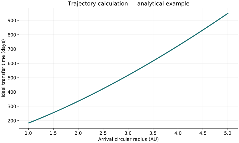
Twenty worked examples

Open a problem to see its defined inputs, assumptions, equation, numerical substitution, result, and interpretation. Values are illustrative analytical exercises.

Connect this subject to other models

• Astrodynamics and orbital mechanics
• Rocket design models
• Satellite design models
• General relativity: geometry, gravity, and matter

Return to the subject library · Numerical solution techniques

Typical sensors and experimental connections

GNSS receiver · Star tracker · Radar sensor

These are examples of instruments used to measure relevant observables, calibrate parameters, or test a physical system. They do not directly measure every abstract model quantity or prove a theory by themselves. Choose bandwidth, range, environment and uncertainty for the actual experiment.

Explore the dedicated Sensors site →

Mathematical tools and foundations

Derivatives and chain rule · Linear systems and elimination · Monte Carlo estimation

Use the stated mathematical conditions together with the physical assumptions. Explore the Mathematics atlas →